Chapter 5 Vocabulary Size

This chapter begins our substantive analysis of properties of language learning and their variation across languages and children. We begin with one canonical view of CDI data, in which each child is represented by a single vocabulary score: the proportion of words that child knows, out of the total in the form. We first quantify the median pattern of vocabulary growth observed in our data; we then turn to characterizing variability across individuals in these data. In these analyses as well as subsequent chapters, our inspiration comes from what we think of as the “Batesian” approach to variation.

Far from simply reflecting noise in our measuring instruments or variability in low-level aspects of physiological maturation, the variations that we will document (in vocabulary development) are substantial, stable, and have their own developmental course. Because this variation is substantial, it is critical for defining the boundary between normal and abnormal development; because it is stable, it provides a window onto the correlates and (by inference) the causes of developmental change; and because it has its own developmental course, it can be used to pinpoint critical developmental transitions that form the basis for theories of learning and change. (Bates et al., 1995)

We are interested in these theoretical uses of variability. But variability is only meaningful in the case that it is stable; that is, that it reflects signal about individuals (or cultures) rather than measurement error. With respect to the CDI, the strong evidence for the reliability and validity of the forms – reviewed in Chapter 4 and in Fenson et al. (2007) – provides support for the contention that observed variability is meaningful. To foreground one of the strongest reliability studies, we note that Bornstein and Putnick (2012) collected multiple language measures at 20 and 48 months in a sample of nearly 200 children and used a structural equation model to estimate the stability of a single latent construct, language ability. Essentially all measures related strongly to this latent variable and the coefficient on its stability over time was r = .84, suggesting that early language is quite stable, at least when measured appropriately. Notably, the ELI, a precursor to the CDI, was included in the measures at 20 months and was found to correlate with the 20-month latent construct at r = .87.

This finding – along with the other evidence, mentioned above – justifies the implicit conceptual model of the following analyses. That model is that there is a single quantity, early language ability, that is stably measured by parent report and that can be approximated as the raw proportion of words a child “understands” or “understands and says” on CDI forms. Such evidence has primarily been collected for the English CDI, however. In this chapter we examine variability across the full set of languages, and it is worth remembering that we project the reliability and validity of the English instrument to its adaptations.

5.1 Central tendencies

The first question we can ask about CDI data is about its central tendency – the median pattern of vocabulary growth. Our general expectation is shown in Figure 5.1.

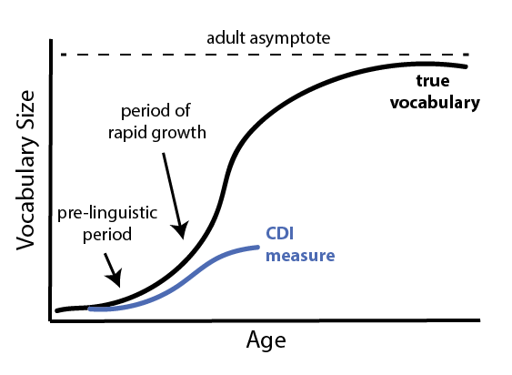
Figure 5.1: Schematic true vocabulary growth and vocbaulary growth as measured by the CDI.

This schematic reveals a number of patterns that are explored in this and subsequent chapters. The CDI necessarily captures a small fraction of any individual’s true vocabulary, but even within the measured range there are a number of specific questions that can be addressed by different analyses. The question of the exact slope of children’s growth, especially in the period immediately after the emergence of language, is treated in Chapter 15 – this question is sometimes posed as whether children undergo a vocabulary “spurt” (Ganger and Brent 2004; but cf. McMurray 2007). On the other side of the CDI curve, the question of the divergence between CDI-measured vocabulary and true vocabulary (and whether true vocabulary can be recovered via a statistical correction) is treated in work by Mayor and Plunkett (2011) – because of the English-specific nature of this work, we do not take up this issue here. In the current chapter, we focus on the middle section of the CDI curve, in which children’s vocabulary is neither at the floor or the ceiling of the instrument.

5.1.1 Commonalities across languages

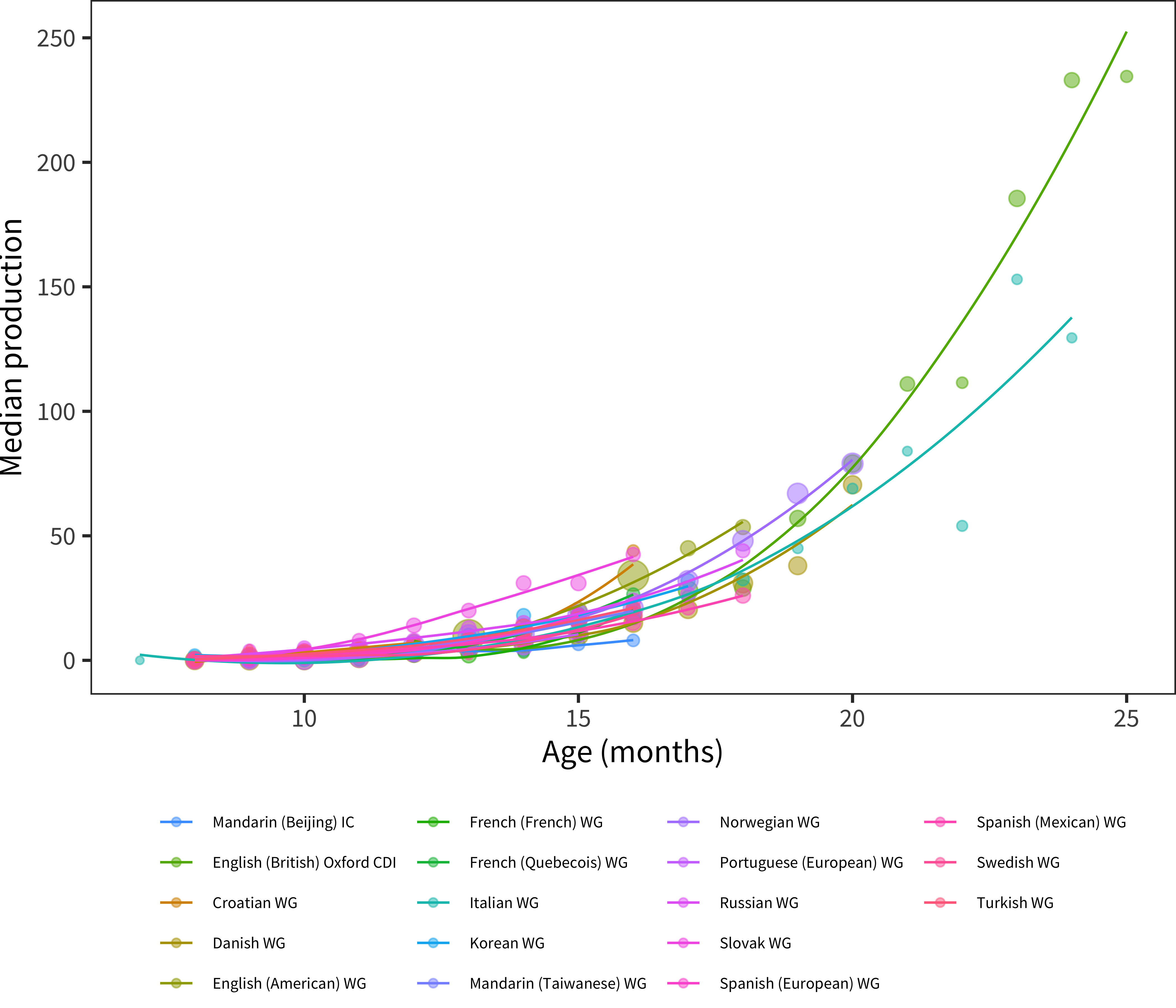
Figure 5.2: Median production using Words and Gestures-type forms. Included are only languages where there are more than 200 administrations total.

Figure 5.2 shows the median patterns of growth for early production. Rather than showing proportions, as we will do more standardly throughout the book, here individual item totals are plotted. In general, the median child before the first birthday is reported to produce a small number of words. (These data raise a number of questions about the specific reliability of very early parent reports, which we take up below.) Overall, however, these curves accord relatively well with our intuitive sense of early vocabulary development: they reveal that most children tend to speak at most only a few words before their first birthday, but that production accelerates across the second year.

This analysis also motivates the decision to omit production data from Words & Gestures forms from moast of the analyses in subsequent chapters. Many WG forms end at 16–18 months, meaning that the median production is only around 50 words. For analyses of vocabulary composition or predictive modeling, these numbers are often too small to yield meaningful cross-item conclusions, although they can be combined with Words & Sentences data (see Appendix C).

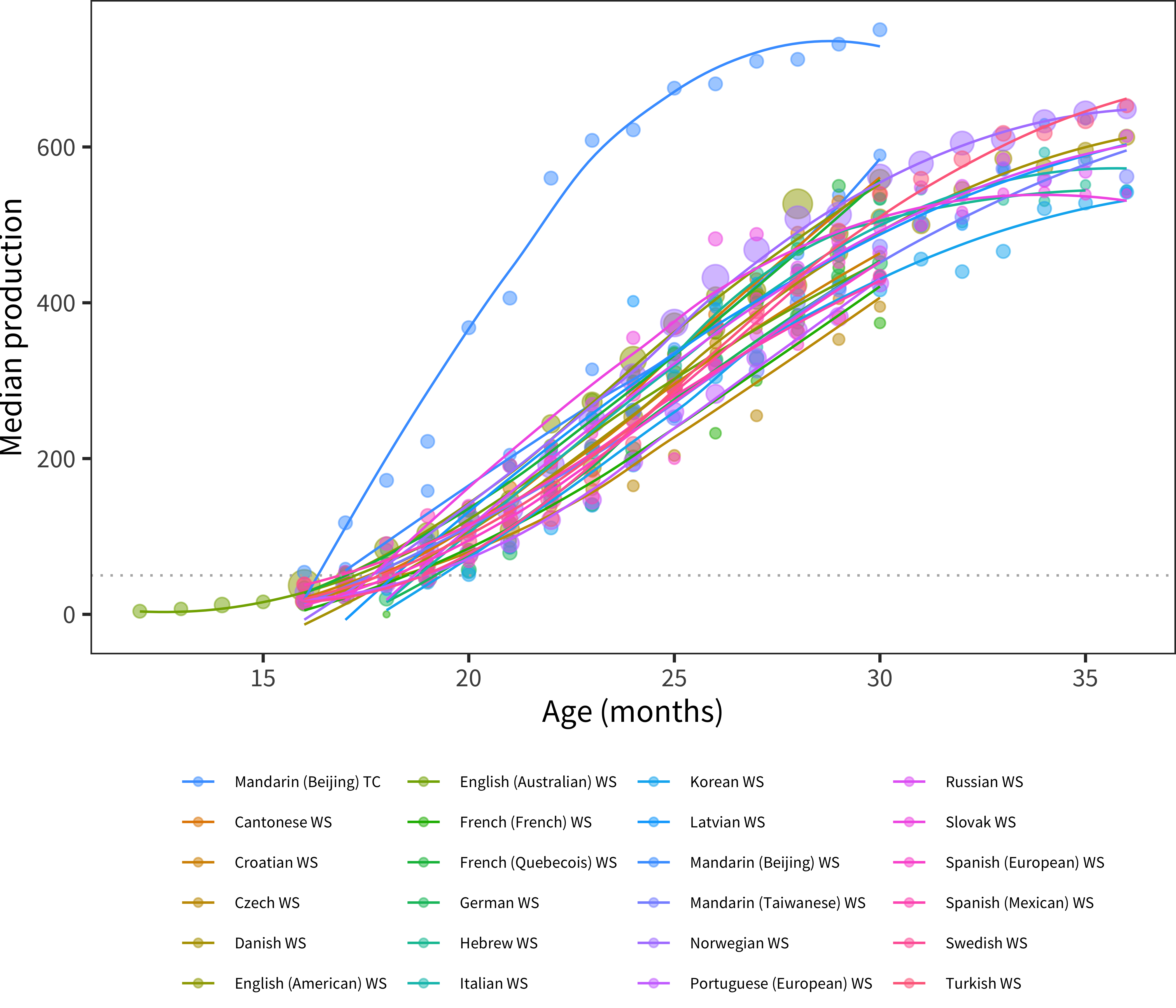
Figure 5.3: Median production using Words and Sentences-type forms. Included are only languages where there are more than 200 administrations total.

The acceleration in early vocabulary is even clearer when looking at production reports from older children using Words & Sentences. Figure 5.3 shows this pattern. In every language, the median child is reported to produce 50 words between 16–20 months (dotted line), though – as we will see below – this analysis masks tremendous between-child variability during this period. In addition, languages vary considerably in the absolute number of words reported. (As it is a major outlier, we have discussed the Beijing Mandarin WS data in Chapter 3, section on difficult data). Nevertheless, there are still substantial consistencies in the shape and general numerical range across languages.

During the period of 24–30 months, we see curves leveling out. Presumably, this leveling does not reflect a slowing in the rate of acquisition, which most researchers assume continues unabated for many years (e.g., Bloom, Tinker, and Scholnick 2001). Instead, it reflects the limitations of the CDI instrument, in that there are many possible “more advanced” words that children are likely learning, of which only a small subset are represented on any form.

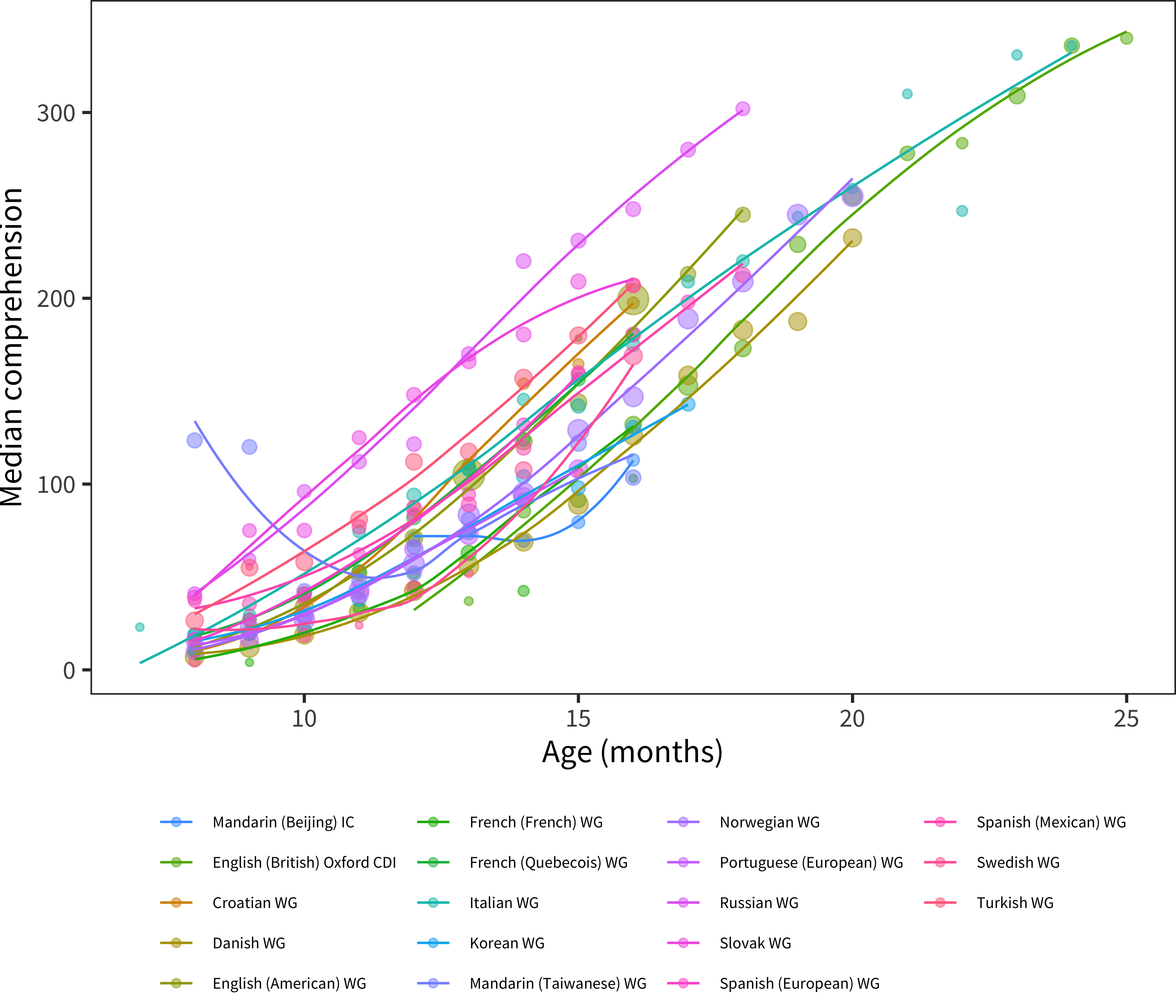
Figure 5.4: Median comprehension using Words and Gestures-type forms. Included are only languages where there are more than 200 administrations total.

We next turn to comprehension medians, shown in Figure 5.4. Comprehension is queried only on the Words & Gestures form. Reported comprehension increases much faster than production; so much so that most parents are reporting that their children understand most words on the form by 18 months (Chapter 15 discusses differences in the balance between comprehension and production between children). As with the production data, we see substantial differences across languages in reported vocabulary, discussed below (see Chapter 3, section on difficult data, for more discussion of Taiwanese Mandarin comprehension data).

One striking aspect of the comprehension data is how early comprehension is reported. For example, from 8 months, we see parents reporting medians of 4.5 (Swedish) and 123.5 (Mandarin (Taiwanese)) words. To many researchers (and some parents) these high numbers feel unlikely. We are largely agnostic on this issue, but the literature does provide some support for early comprehension reports. A spate of recent infancy experiments suggest that in fact, children in the second half of the first year do have some fragmentary representations of many common words available (e.g., Tincoff and Jusczyk 1999, 2012; Bergelson and Swingley 2012; Bergelson and Aslin 2017). The representations revealed in these tasks are quite weak – often amounting to a 2-5% difference in looking to a target on hearing a word uttered. Despite its weakness, depending on the criterion used by parents, this knowledge may be what is detected in these early reports. Thus, these estimates may not be as far off as we initially supposed.¹²

5.1.2 Cross-language differences

Setting aside outlier datasets, there is other variation between languages apparent in the preceding analyses. To what extent is this variation meaningful? We explore this question next, focusing on production data from the Words & Sentences form, as these data are the densest and most reliable. We consider a range of explanations in turn.

1. Differences could be due to differences in form length. As shown in the plot above, however, medians for proportions and raw scores are highly correlated (r(22) = 0.906, p < 0.001), suggesting that the ordering of languages is not only a function of form length. Raw scores have a positive but non-significant correlation with form length (r(22) = 0.336, p = 0.11); this correlation changes direction and is not reliable for proportions (r(22) = –0.079, p = 0.71). In sum, it appears that there are form-length differences (motivating the use of proportions in general), but that there is still variation between languages even correcting for this issue. Figure 5.5 shows the relevant proportion trajectories, highlighting remaining differences between English and Danish (two languages for which we have substantial datasets with full demographic information). As Eriksson et al. (2012) write, “Using raw data assumes that each form is exhaustive, while using percentages assumes that each form is equally exhaustive. Neither is correct and the truth lies somewhere in between.”

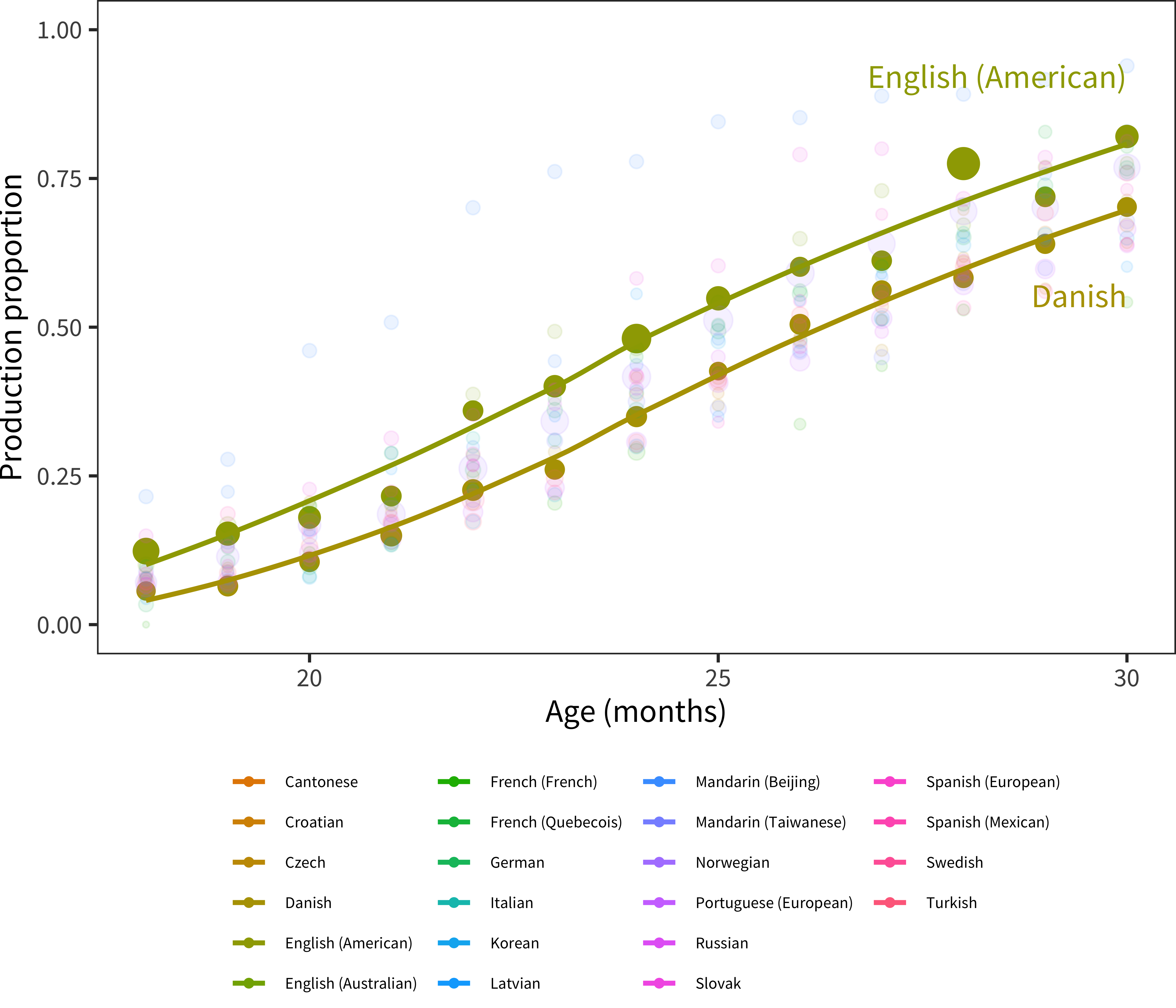
Figure 5.5: Cross-linguistic production data, proportions plotted by age. English (American) and Danish are highlighted.

2. Differences could also be due to form construction. For example, the Czech form could select relatively harder words for inclusion, leading to fewer words being checked. We cannot directly address questions about the difficulty distribution of items without moving to psychometric models (see Chapter 4). These models in turn would need to be equated across forms in order to compare latent ability scores across instruments. While we have experimented with these procedures, there is a circularity to test equating procedures that makes us leery of proceeding. In particular, in order to equate across tests in standard item response theory models, it is critical to have test items that are shared across instruments. But although we have concepts that are shared across instruments (see Chapter 10), we do not believe the words that represent these concepts are necessarily equally difficult across languages – in fact, the premise of some of our later analyses is that they are not. Thus, assessing form difficulty across languages is a complex proposition that we do not address directly here.

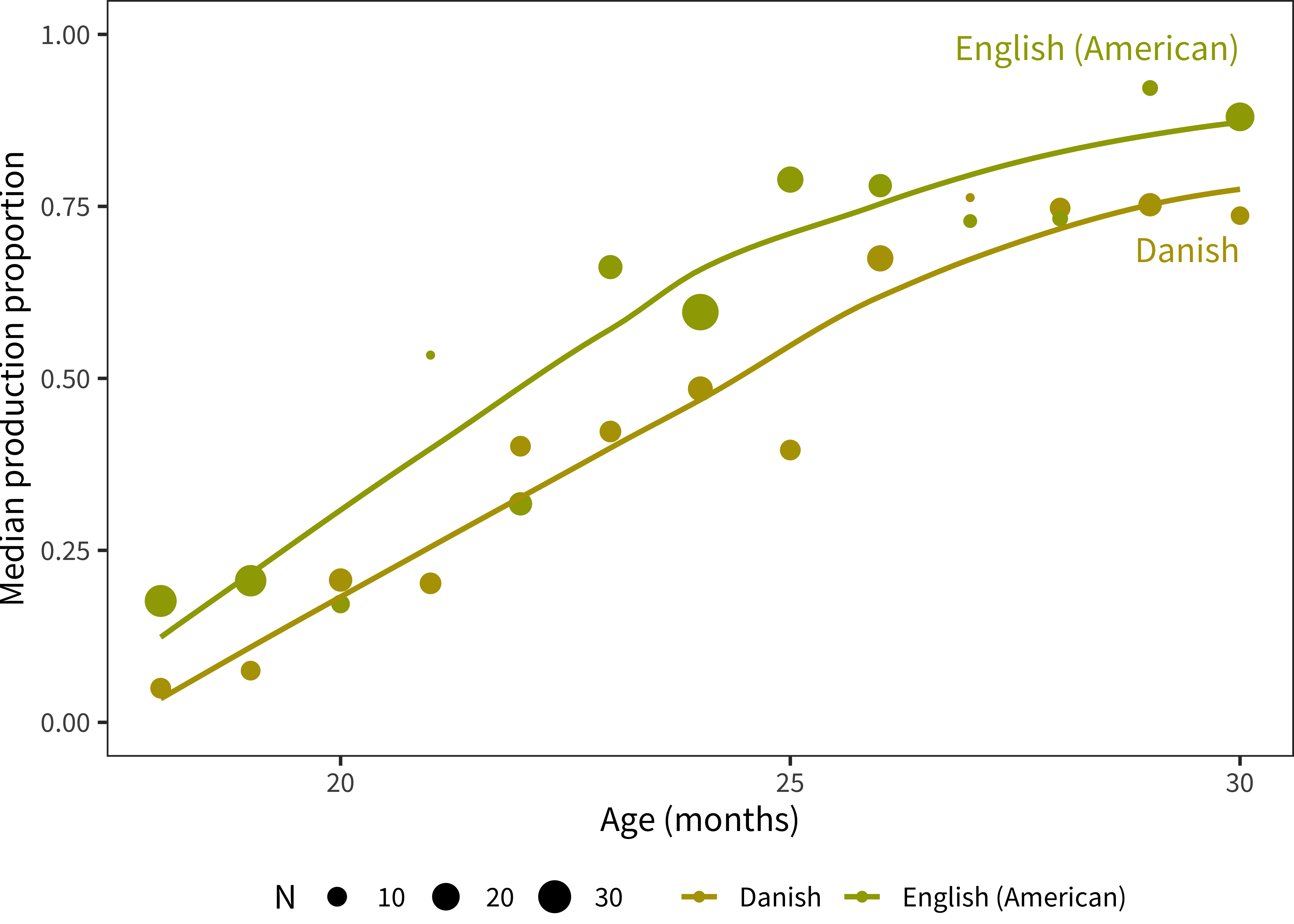
Figure 5.6: Proportion production plotted by age for Danish and English samples, now subsetting to the first-born female children of college-aged mothers.

3. Differences could also be due to demographic differences across samples. We have examined sample composition in Chapter 3 and see that – to the extent we have access to demographic data – sample composition does vary in features that affect vocabulary (e.g., maternal education, birth order; see Chapter 6 for fuller analysis). We are not yet in a position to conduct a full analysis of these differences, controlling for demographics, as data are sparse and the nature and extent of demographic differences also vary across cultures. Nevertheless, we can note, for example, that differences between Danish and English (American) children look quite similar (though noisier) in female, first-born children of college-educated mothers (Figure 5.6). This would suggest that demographic differences cannot fully explain the cross-linguistic differences that are observed.

4. Differences could be due to cohort effects, in which older sets of data show differences from newer datasets. Most of our data date from the period 2005-2015, but some of our English and Spanish data are older, as they date to the period in which CDI forms were first being designed (the early 1990s; Fenson et al. 1994). Unfortunately, we do not have reliable information about the collection date for many datasets, so we cannot use this variable in regression analyses. Naively, we would expect later cohorts to show higher vocabularies, consistent with the Flynn effect (Flynn 1987). Yet, the Danish data, for example are relatively recent and were collected online using standardized instructions. Danish is subject to its own issues (see below), but the Norwegian data are also relatively recent and are quite comparable to the English data.

5. Differences may relate not to demographics of the sample but to the procedure at administration. These differences are not transparent to us in all cases, and so, similar to cohort effects, we cannot control for them statistically. For example, instructions at administration – whether written on the form or given by experimenters – might have been more liberal in the case of Slovak or English (American) samples. Such instructions could have emphasized completeness in reporting vocabulary. Or the circumstances of administration could have been different – for example, Danish data were collected online while most English (American) data were collected using paper and pencil forms. English (American) data are contributed by many different labs, so there are likely many different administration styles represented.

6. Differences could be due to cultural or experimental differences in reporting bias. Slovak parents might have a lower criterion for reporting knowledge of a word. Following our discussion in Chapter 2, we could speculate that Slovak parents’ model of children’s overall competence might be higher. (Such an explanation could be true in principle for the case of the Mandarin and Hebrew data discussed above, as well, though this would be a case of extreme differences!) This explanation is an extension of the discussion above of administration and instructions – perhaps the relevant differences are in cultural expectations for what it means to be producing a word or for how verbal children are expected to be.

7. Finally, differences could be due to true differences in language acquisition. While this explanation is a possibility, we hope we have emphasized that it is only one among the many enumerated here. Nevertheless, one reason we have emphasized the Danish/English comparison above is that many researchers working on Danish believe that, due to its phonological properties, it truly is a difficult language to learn (Bleses et al. 2008; Bleses, Basbøll, and Vach 2011). In particular, Danish is characterized by some highly distinctive phonological reduction processes which greatly reduce the frequency of obstruents, and more generally lead to “an indistinct syllable structure which in turn results in blurred vowel-consonant, syllable and word boundaries [where]… word endings are often indistinctly pronounced” (Bleses et al., 2008, p. 623). The authors of this study also able to provide evidence against the alternative view that Danish parents are simply more reluctant to respond “yes” – there were no differences on either gestures or word production. They conclude that the phonological structure of Danish produces an initial obstacle to breaking into the stream of speech and is reflected in overall patterns of vocabulary development. While this generalization may in fact be true, research is still needed to explore what other factors might converge to make language acquisition relatively easy vs. hard in some languages than others.

In summary, differences between languages in the sheer number of words reported are unlikely to be accounted for purely by differences in form size or demographic differences between samples. In our (very speculative) synthesis of the preceding discussion, they likely result from a combination of cultural attitudes towards children’s language, differences in administration instructions, and real differences in learning across languages. Partialling out these differences would likely require better-controlled data collection that included constant administration and sampling methods. For this reason, in the remainder of our analyses, we attempt to avoid interpreting overall differences in vocabulary size as much as possible and limit ourselves to quantities that can be effectively normalized.

5.2 Variability between individuals

We next turn from central tendencies in early vocabulary to the issue of variability, one of the most important features of early vocabulary development (Fenson et al. 1994). Across every language in the database there is huge variability in the vocabulary sizes reported for individual children, even within an age group. How can we characterize this variability? That is the question addressed by our next set of analyses.

5.2.1 Quantifying variability

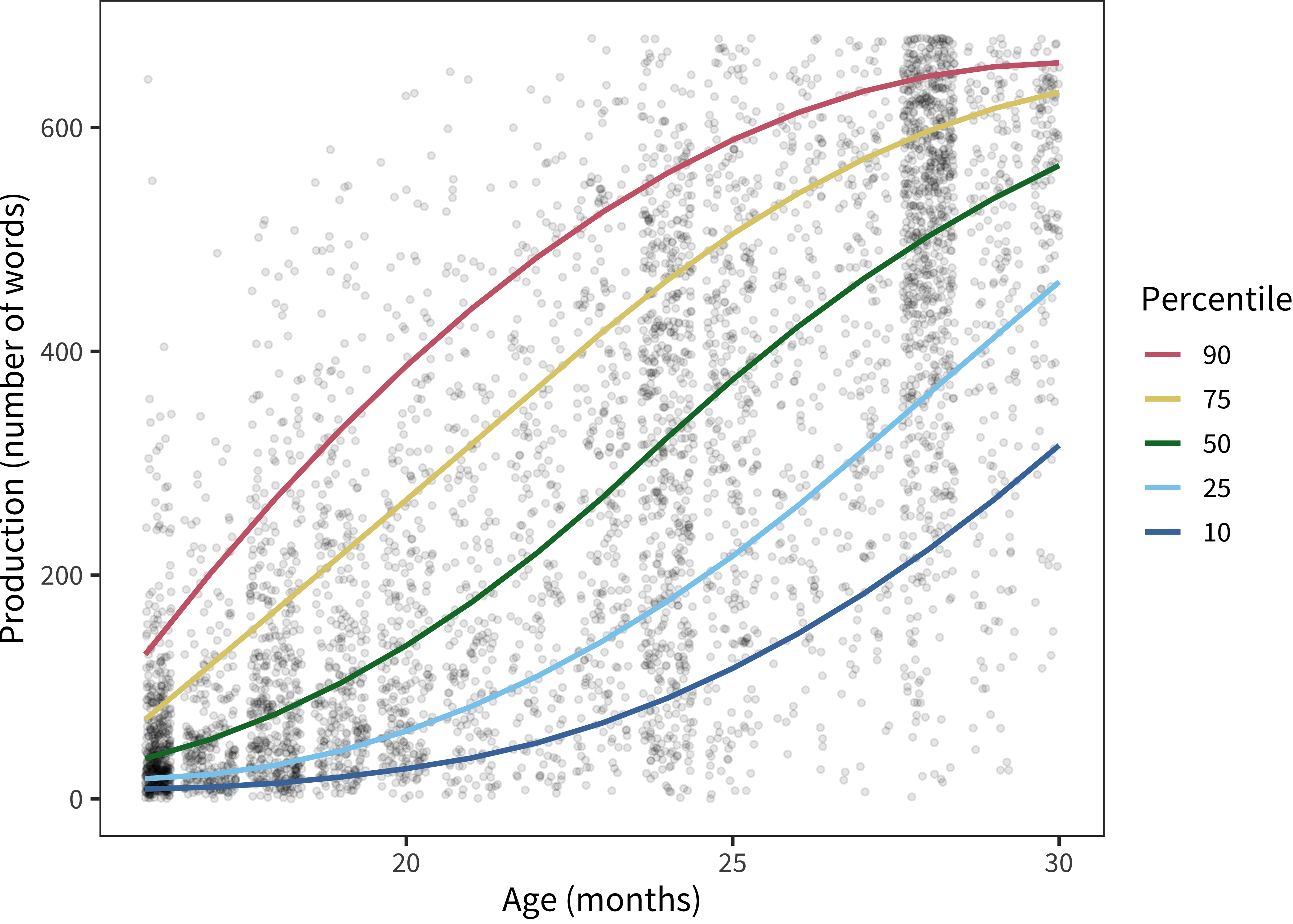
Figure 5.7: Raw production scores for English (American) production data. Dots show individual participants, while lines give standardized percentiles, computed via spline-based quantile-regression.

As an example, we zoom in on the English (American) production data from the Words & Sentences form. The canonical view of these data is given in Figure 5.7. It is very clear that variability is the norm! There are children clsose to the floor and ceiling of the instrument at almost all age groups.

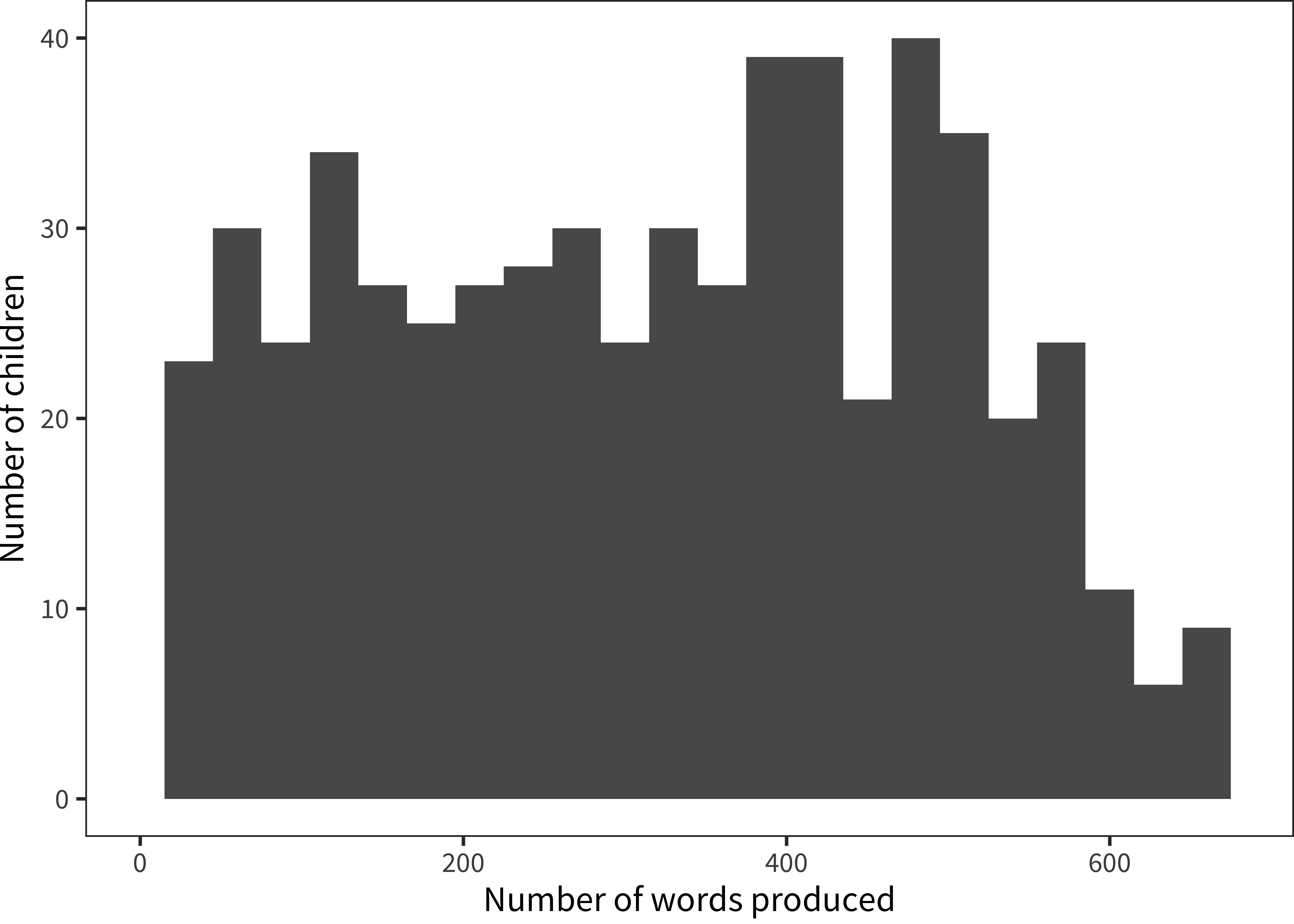
Figure 5.8: Histogram of English (American) production values for 24-month-olds.

We zoom in even further to consider just a single age group, 24-month-olds. A histogram of production vocabulary for this group is shown in Figure 5.8. The distribution of vocabularies across children is far from normal, with many children at the very bottom of the scale and almost as many at the top. In other words, quite a few two-year-olds on their second birthday are reported to produce only a handful of words and others are producing nearly all of the 680 listed on the form.

One way to describe these data is to consider the relationship of the variance to the central tendency. The “coefficient of variation” (CV) is a common measure used for this purpose (with \(\sigma\) denoting the sample standard deviation and \(\mu\) denoting the sample mean):

\[CV = \frac{\sigma}{\mu}\]

This statistic allows us to compare variability across measurements with different scales, an important concern when we want to compare forms with very different numbers of vocabulary items. For example, for two-year-olds, the mean productive vocabulary is 319 words, and the standard deviation is 175 words, leading to a CV of 0.55.

But, again as seen in Figure 5.8, the distribution of productive vocabulary scores is far from normal. And, distributions deviate even more from the standard normal distribution at younger and older ages. Thus, a non-parametric approach is more appropriate. Accordingly, we compute the MADM statistic, the non-parametric equivalent of the CV (Pham-Gia and Hung 2001). In MADM, the mean \(\mu\) is replaced by the median (\(m(x)\), and the standard deviation \(\sigma\) is replaced by the mean absolute deviation (which captures how far away values are from the median):

\[MADM(x) = \frac{\frac{1}{n} \sum_{i = 1..n}{|x_i - m(x)|}}{m(x)}\] Appendix B demonstrates that, although MADM is more appropriate for our data, CV and MADM are very highly correlated with one another across CDI datasets.

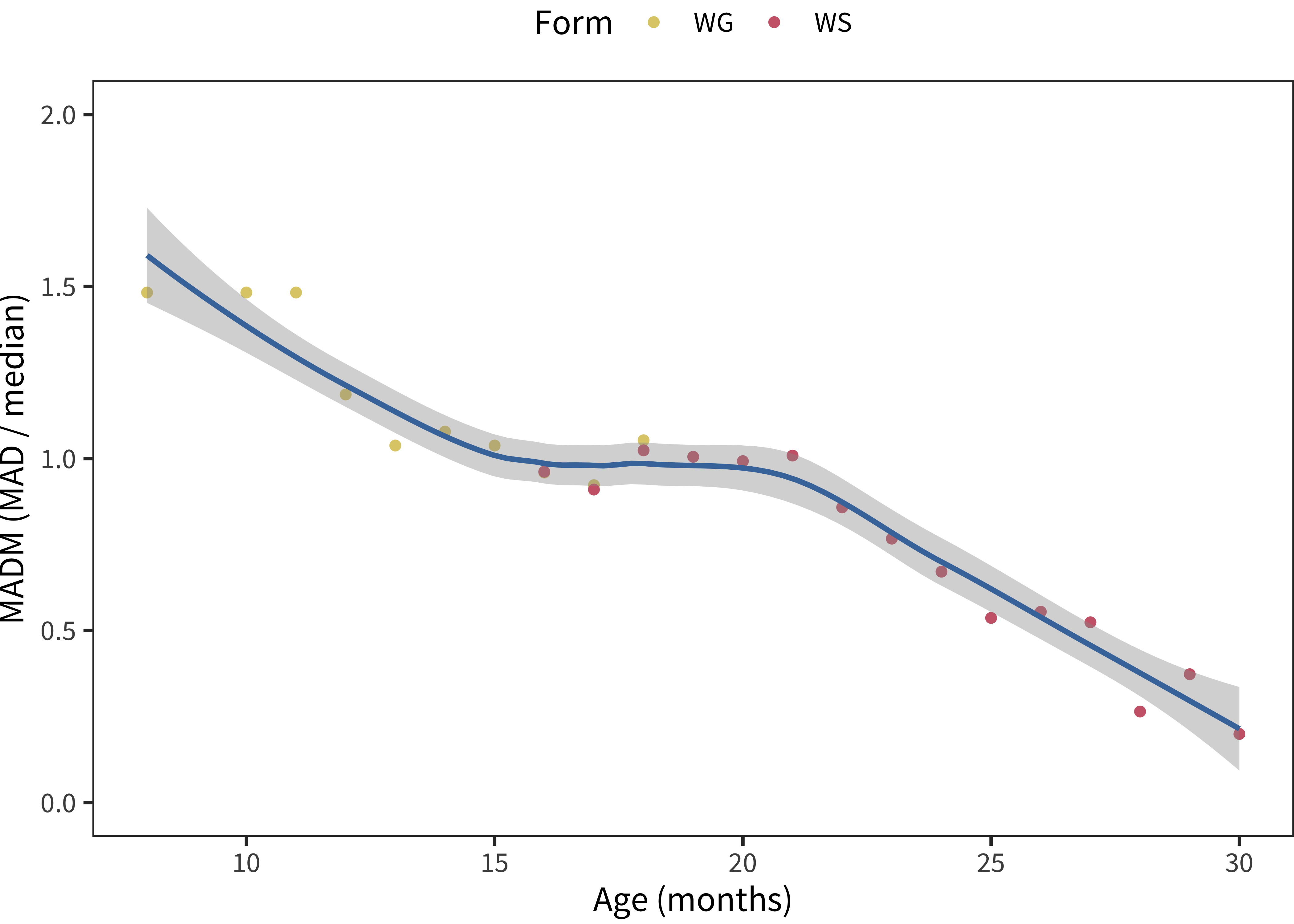
Figure 5.9: MADM values plotted by age for English (American) production data, across forms. The smoothing line is produced by a loess smoothing function.

Figure 5.9 shows the MADM value for American English production data, plotted by age. In these data, the MADM is actually close to 1 from age one until almost age two, suggesting that the standard difference from the median is actually as big as the median itself!

To get a sense of this variability, it can help to have a smaller dataset to consider. Imagine groups of three children. A group where one produced 30 words, one produced 100, and another produced 170 would have a MADM of 0.99. In contrast, one where they were more closely grouped – say 70, 100, 130 – would have a MADM of 0.44.

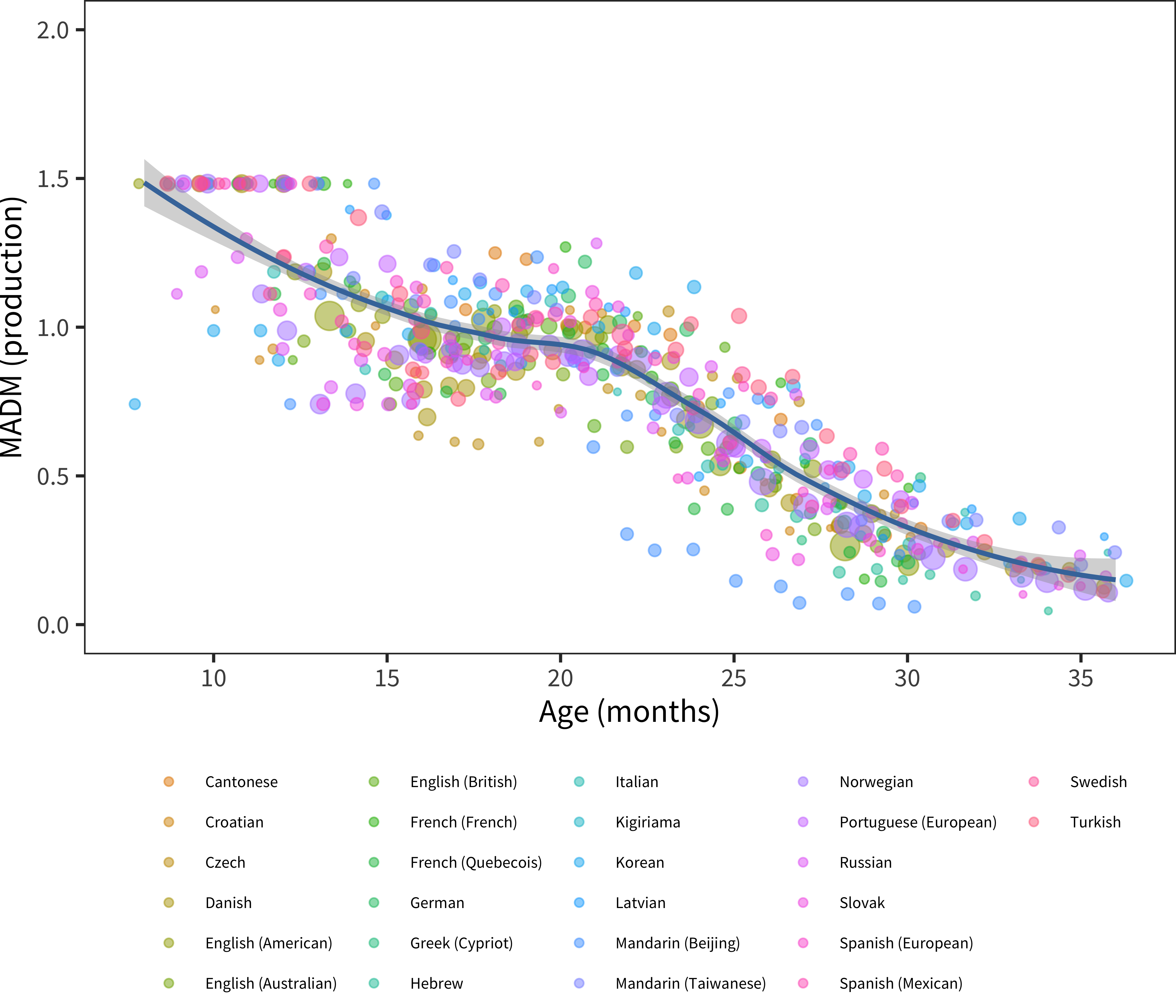
Figure 5.10: MADM for production, plotted by age group, for the full sample of languages in our dataset.

Does the general level of variability observed in American English hold for other languages? Figure 5.10 shows the MADM for production across languages and instruments. This similarity in variability is quite striking. Between the first and second birthdays, children’s early language is remarkably variable, but this variability itself is quite consistent across languages.

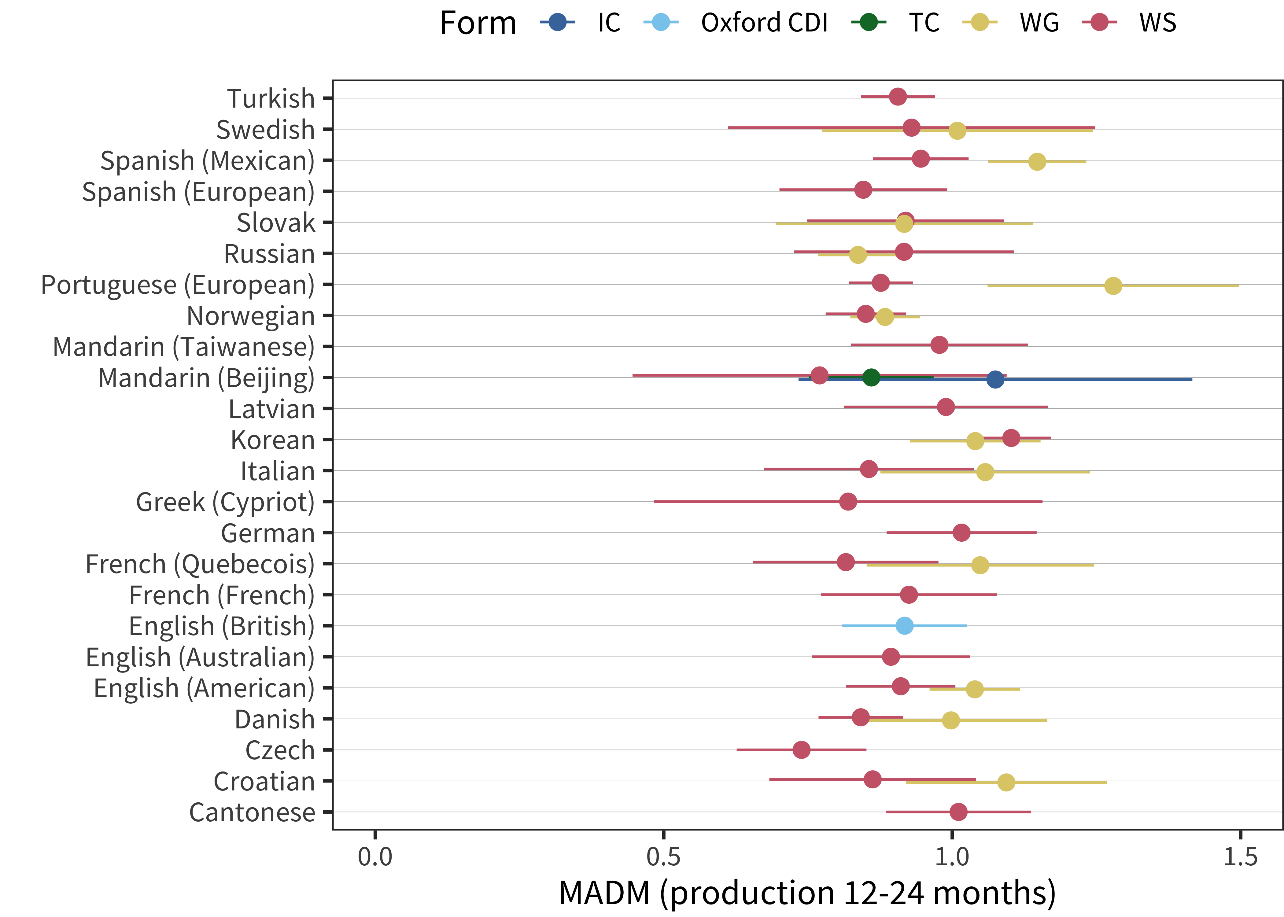
Figure 5.11: MADM values from 12-24 months for all languages and forms.

We summarize the MADM in the second year of life by taking its mean across that age range. This summary is shown in Figure 5.11. The MADM mean is close to 1 for almost every language and form for which we have data. In sum, confirming the analysis above, we see strong cross-linguistic consistency in the variability of children.

One question that could be raised regarding the analysis above is the extent to which variability is caused by variability across children vs. variability in reporting. The extreme values seen in the English data, for example, could conceiveably be the result of a mixture of lazy parents who stopped answering the form with overly diligent parents who misunderstood and checked every box for a word they thought the child had been exposed to. But, to the extent these biases are the source of variability, they are extremely consistent across languages – which, recall, is the exact opposite argument from the one we considered above (where parent diligence was supposed to be variable enough across samples to lead to differences between languages).

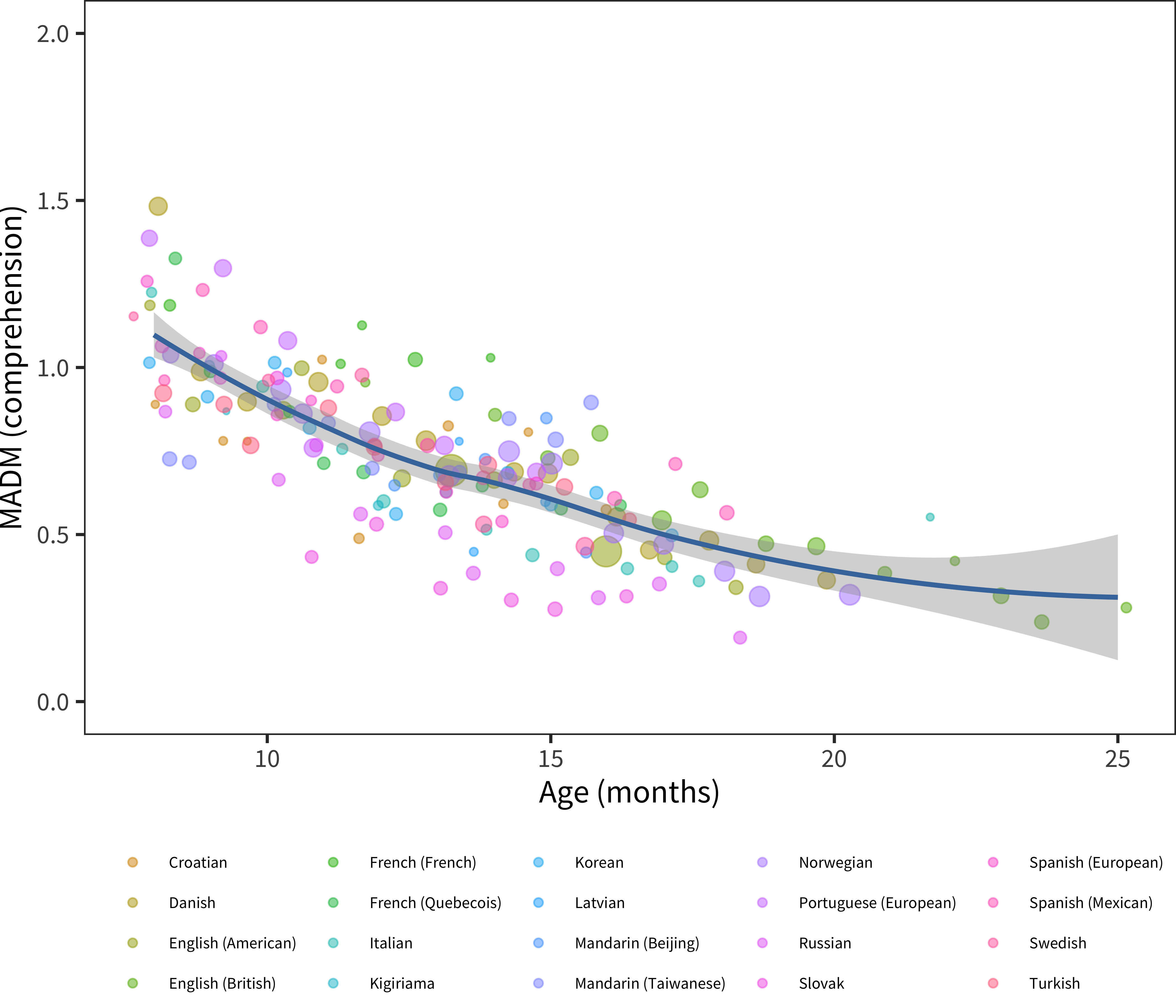
Figure 5.12: MADM for comprehension, plotted by age group, for the full sample of languages in our dataset.

The same analysis for comprehension data is shown in Figure 5.12. For comprehension, we see a gradual decrease in variability throughout development. The intercept for the 12-18 month period appears to be lower than that observed in production, despite – or perhaps due to – higher comprehension scores. This observation matches one made by Mayor and Plunkett (2014), namely that, across children, production vocabulary appears more idiosyncratic than comprehension vocabulary. One speculative explanation for this difference would be the tremendous differences in speech-motor development (as well as general differences in loquacity) between toddlers (for an example, see Clark 1993). This variability would then carry over into production vocabulary size. Another possibility, however, is that true variability is masked by the overall lower reliability of comprehension items (see Chapter 4). Our data do not allow us to distinguish between these two explanations.

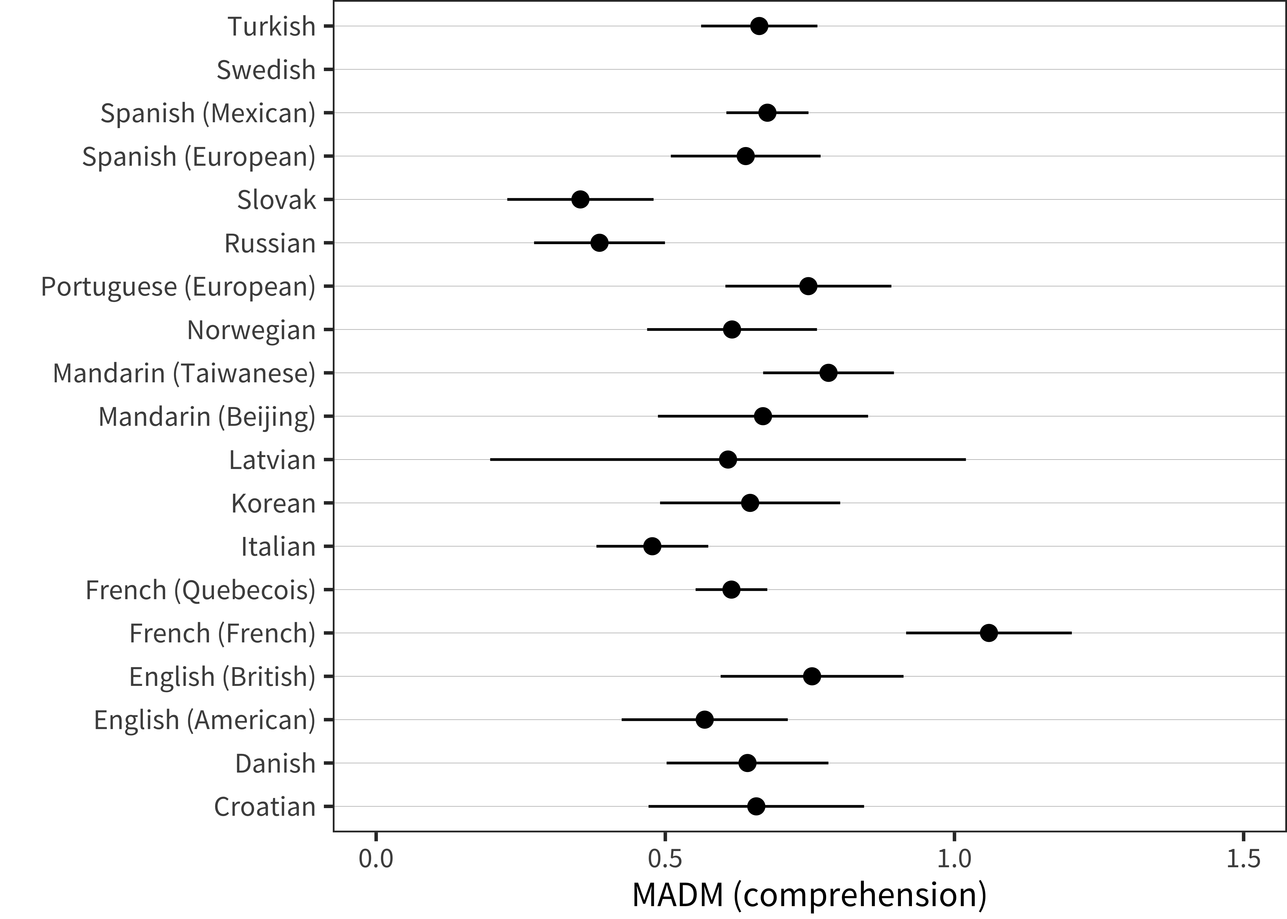
Figure 5.13: MADM values from 12-18 months for all languages and forms.

The final plot in this sequence is shown in Figure 5.13, which shows 12-18-month average comprehension MADM values. These are slightly lower and slightly more variable than the production values shown above, but still display a quite consistent level of variability.

5.2.2 Is there a ceiling to variability?

The analysis above suggests that variability between individuals decreases. But this conclusion is compromised by ceiling effects: once children begin to reach the ceiling of the CDI form, variability is necessarily truncated. No analysis can completely eliminate these effects, but the use of item response theory-based analyses can partially address the issue by estimating variation in latent ability rather than variation in raw scores themselves.

Chapter 4 provided a summary of our approach to using item response theory (IRT) with CDI data. In brief, IRT provides a framework in which the full test (the CDI) is analyzed as a series of items, with each having its own logistic model predicting the response for a particular child on the basis of their latent ability. In Chapter 4, we examined the parameters of individual items with respect to their properties; but fitting an IRT model also implies estimating a set of latent ability parameters for individual participants. These latent ability parameters are logistic regression coefficients and hence are not bounded in the same way that individual responses (and hence raw scores) are. Thus, we can examine their variability as a way of dealing with ceiling effects.

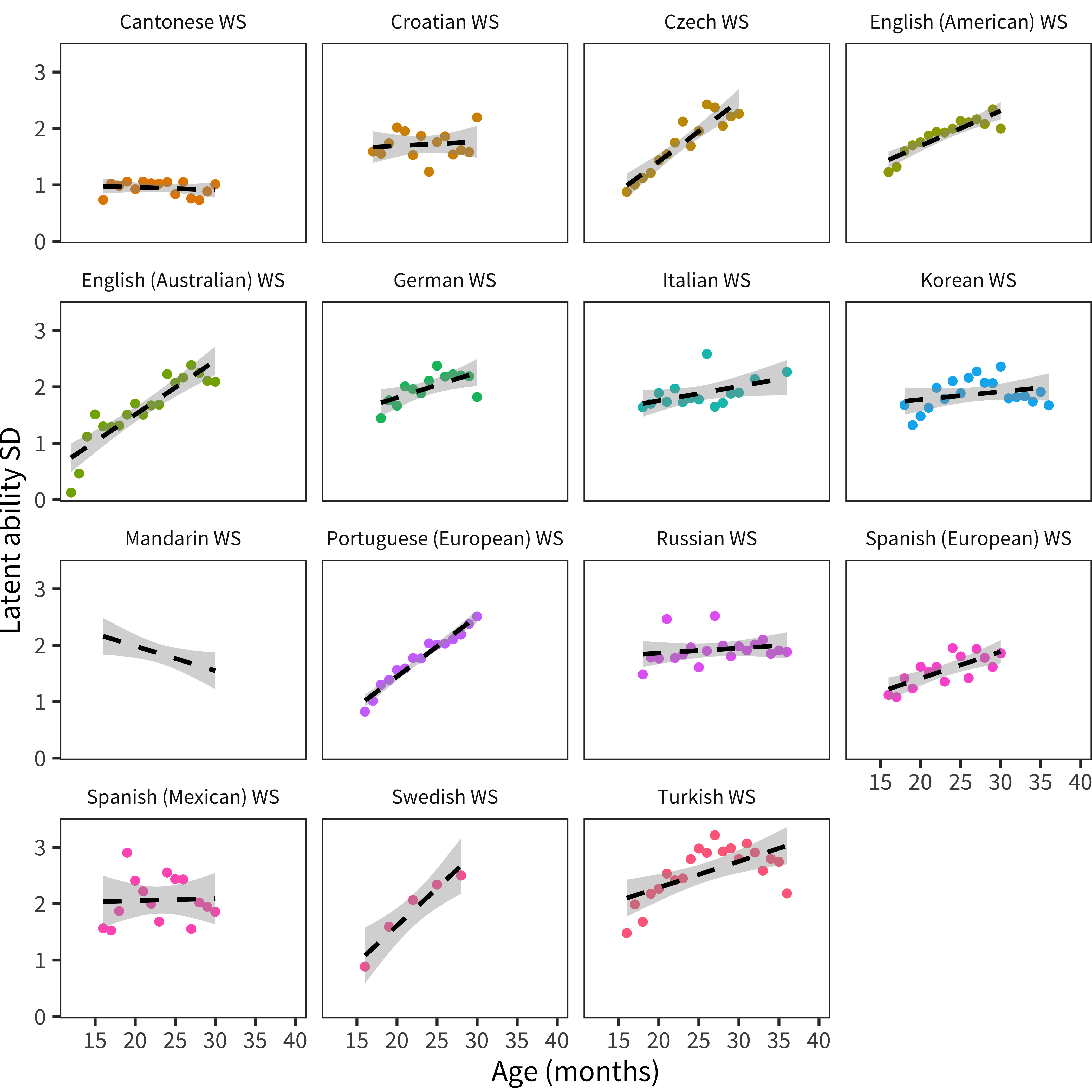
Figure 5.14: Standard deviation of latent ability scores from 4PL IRT models fit to each Words and Sentences-type dataset. Panels show individual languages. Smoothing lines are linear model fits.

We fit a 4PL IRT model to each dataset and estimated the resulting latent ability scores for each child. We then conducted the analysis above, substituting latent ability scores for raw vocabulary scores. Figure 5.14 shows the normalized standard deviation of latent ability scores, plotted by age. The absolute size of the standard deviations is not easy to interpret – the range of latent ability scores on a form is a function of how consistently difficult or easy the items are (and as we noted above, we do not think it is trivial to equate these scores across tests). Thus, the standard deviation of these scores is not comparable across models.

On the other hand, age-related trends in the standard deviation are interpretable and can be used as an index of whether variability in ability stays constant, increases, or decreases. Across datasets, age slopes for the variability of latent ability tend to be flat or even increasing (with Mandarin, which has extreme ceiling effects, being the exception). This finding suggests that the developmental decreases in variability observed above are very likely due to ceiling effects. When we remove these ceiling effects, we find that variability is constant – or perhaps even increasing – throughout the full measured range of early language.

5.2.3 Discussion

We have observed a striking consistency in the individual variability of children’s vocabulary during their second year and perhaps beyond. Across languages and forms, it appears to be the norm that toddlers vary.

What does it mean to have such a high level of variability? For one comparison, we compare age of walking onset (as measured by a Norwegian national survey with parent 47,515 respondents) and age of achieving production and comprehension milestones (also in Norwegian). Walking data are from Størvold, Aarethun, and Bratberg (2013).

Table 5.1: Comparison of language milestones with walking. 25th and 75th give the ages at which that percentile ranking is achieved; ranges give the interval between 25th and 75th percentile in months and as a proportion of total age.

Response	25th	75th	Range (months)	Range (prop)
walking	12	14	2	0.15
produces 10 words	13	16	3	0.21
produces 50 words	17	20	3	0.17
produces 100 words	18	23	5	0.25
understands 50 words	10	15	5	0.42
produces 200 words	20	26	6	0.26

Table 5.1 shows the 25th and 75th percentiles for walking and several language milestone behaviors. The spread of achieving walking (defined as taking a step independently) is quite tight with a mean of 12.9 months and a spread of only a month between 25th and 75th percentile. Very early language comprehension and production are relatively similar with 2 and 3 month spreads. In contrast, construed as milestones in this way, production and comprehension of larger numbers of words each have quite a large spread in comparison to walking (even as a percentage of age).

In sum, our results echo the conclusions of Bornstein and Cote (2005) based their comparative study of Spanish, English, and Italian. They noted that “individual variability is probably a universal feature of early language acquisition” (p. 311).

---

12. An alternative possibility is that both accounts are true, but unconnected: 8-month-olds could in fact know some common words, but parents could be overestimating their vocabulary based on observed behaviors – in essence, parents could be right, but for the wrong reasons (Bergelson and Swingley 2015).↩︎