Chapter 16 Variability and Consistency Within and Across Languages
In each of the analytic chapters of this book (roughly speaking from Chapter 5 to 15), we have presented analyses of specific phenomena of theoretical interest. Wherever possible, we have generalized these analyses across languages so that their relative consistency can be examined and discussed. This chapter brings together a selection of the analyses from these different chapters into a single analytic framework, implementing the general idea discussed in Chapter 1.
In outline, we identify “signatures” for each of the preceeding chapters: measurements that we believe are theoretically interesting or central. We then quantify variability in these signatures across languages, using a single measure. These estimates of cross-linguistic variability quantify the degree to which aspects of language development are more or less similar across different languages and cultural contexts. While there are some limitations to the method we employ, this method nevertheless allows us to synthesize results across very disparate analytic frameworks and methods.
16.1 Analytic method
We begin by identifying a small number of measures computed in each chapter to serve as the “signatures” to be promoted into this analysis. For each measure, we compute its cross-linguistic variability using a standardized measure of variance, the coefficient of variation (CV), where \(\mu\) is the mean and \(\sigma\) the standard deviation:
\[CV = \frac{\sigma}{|\mu|}\]
This measure can range from 0 (indicating a phenomenon that is completely invariant across languages) to infinity (with higher numbers indicating greater variation). The CV provides a single common measure to allow comparability of otherwise very different quantities, allowing inferences across analyses and datasets.
Each measure for which we compute the CV will have both a different base unit and a different number of languages contributing. For example, when considering the correlation between grammar and the lexicon (Chapter 13), we will compute the CV of a set of \(r^2\) values over languages. In contrast, when we look at the size of the noun bias (Chapter 11), we will be looking at a bias estimate that also ranges from -.5–.5 and is typically much closer to 0, computed over 27 languages. To assist in interpretation, we include only those measures that can be computed in 6 languages or more; provide the N contributing languages for all analyses; and compute an estimate of the standard error of the CV (\(SEM \approx CV / \sqrt{2N}\)).
The set of signatures we include in this analysis are necessarily a subjectively-determined subset of the possible measures we have examined in the book. And, of course, those in turn are a subset of the measures we could have computed. Wherever possible we have attempted to make reasonable decisions, but some of these are, by necessity, somewhat arbitrary. An example of such a decision comes from the summary of Chapter 5. In that chapter we noted that population variability appears quite consistent across languages. We summarized population variability in production via a statistic, MMAD – but what is the appropriate range of ages to include in a single estimate? We also observed that there appears to be a ceiling effect in the later ages. Thus, we decided to include variability in production from 12 – 24 months. But this decision is data-dependent and so, of course, there is a risk of circularity. We point the issue out not to undermine this particular analysis; we believe the ceiling effect is quite clear and other aspects of the age choice do not lead to much change in the CV estimate. Rather, we intend to highlight that the summary we give is not a theory-neutral estimate but rather a “best guess” – an attempt to navigate the myriad choices involved in our analysis in a reasonable way.
One example of such a choice is that we have made the decision throughout to omit estimates of early production from WG-type forms. Our judgment was motivated by the fact that such estimates are routinely quite noisy and difficult to interpret, likely due to the small size of early productive vocabularies. In chapter after chapter, we found unreliable or uninterpretable results that are plausibly due to data sparsity; thus, we choose to omit these patterns from our broader synthesis effort.
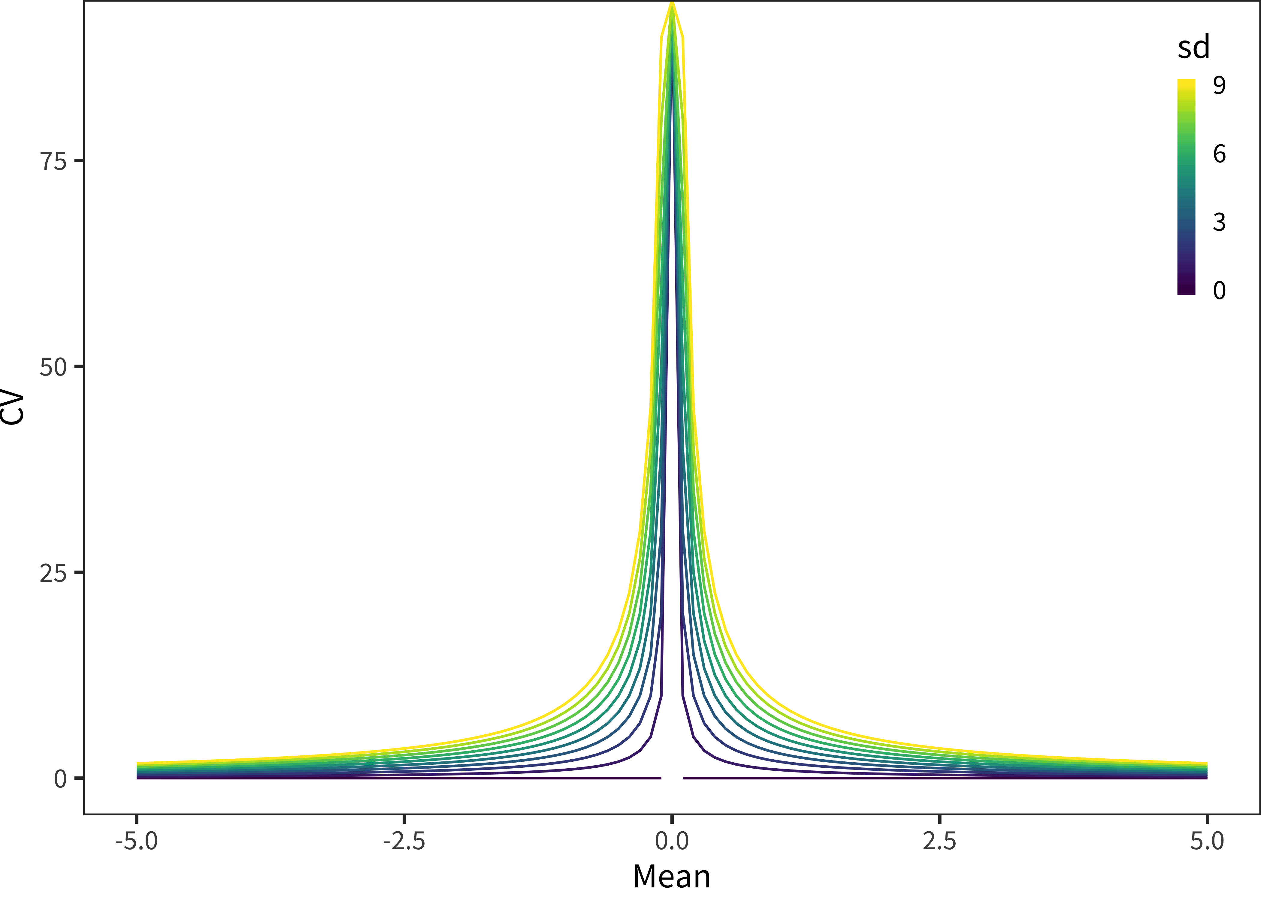
Figure 16.1: A theoretical analysis of the properties of the coefficient of variation (CV) method. CV is plotted by its two components: mean and standard deviation (sd). Mean values are shown on the horizontal axis, with colors indicating different standard deviations.
One key interpretive caution comes from the nature of the CV measure, however. The goal of the CV measure is to provide a unit-less way to compare variability across many measures. But because it is a ratio, when \(\mu\) is small, CVs can be arbitrarily large. Figure 16.1 shows this relation. Concretely, this property will cause difficulties for us when we have phenomena within a particular grouping that have both small means and small standard deviations relative to other phenomena. For example, in Chapter 12, the bias for household words is negligible – as is the variation across languages. But, because the mean bias is very close to zero, the coefficient of variation appears gigantic. To assist interpretability, we have simply omitted negligable effects like this from the analysis below, recognizing that this move limits the generality of the approach.
16.2 Results and discussion
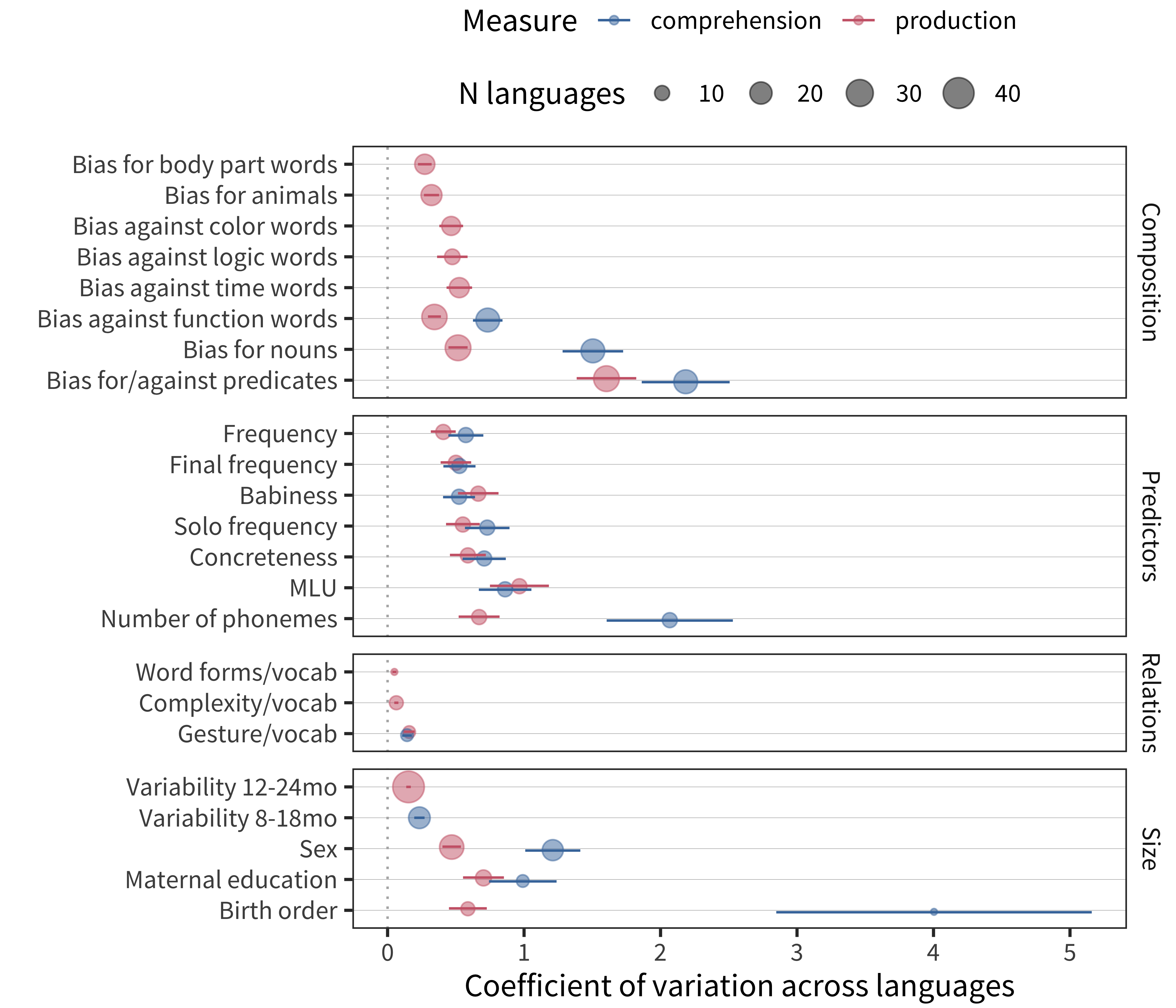
Figure 16.2: Coefficient of variation across languages for signatures of language development corresponding to four different categories (panels). Each point gives an estimate, with point size corresponding to number of languages. Color indicates whether comprehension or production is measured. Error bars give the standard error of the coefficient of variation.
Figure 16.2 shows the coefficient of variation across languages for selected measures. For the sake of our analysis, we have divided measures from the preceding chapters into four categories. These are:
Measures of the composition of vocabulary, from Chapters 11 and 12. These measures describe the over- and under-representation of various word categories in vocabulary. The units over which the CV is computed are bias scores; these are bounded from -.5 to .5 (deviation from unbiased acquisition of a particular category).
Predictors of word difficulty, from Chapter 10. The consistency of different regression predictors of age of acquisition are represented here by their cross-linguistic consistency. This analysis is distinct from the analysis presented in that chapter (which focused mostly on the magnitude rather than variability of the coefficients themselves). Despite that, we include it here for comparison with other signatures. The units over which CV is computed are standardized regression coefficients.32
Relational measures, from Chapters 7 and 13. These measures are originally correlations between vocabulary size and other aspects of early language.
Vocabulary signatures, from Chapters 5 and 6. These measures document patterns in the overall size of vocabulary across individuals and demographic groups. The original units are themselves variability-based (MMAD scores).
A number of local patterns are immediately apparent. First, comprehension is almost always more variable than production, even when a comparable number of languages are included. Why would comprehension be more variable across languages than production, especially given evidence that comprehension vocabulary tends to be less idiosyncratic than production (Mayor and Plunkett 2014)? One strong possibility is the psychometric properties of comprehension vs. production reports. As described in Chapter 4, while comprehension scores are likely still a reliable and valid index of children’s abilities in the aggregate, individual comprehension questions tend to carry less information. Thus, there may simply be more noise in these measurements, leading to less cross-linguistic stability. This regularity illustrates a point we made in Chapter 1: the inferences from consistency and variability are asymmetric. In the case of consistency, we can make relatively strong inferences about some kind of shared process or mechanism. In contrast, in the case of variability, there are many sources of variance (including measurement error) that can account for a specific pattern of performance.
Second, relational measures are highly invariant across languages. These relations include correlations between the size of children’s lexicon (in production or comprehension) and measures of gesture, morphology, and grammatical complexity. These findings can only be measured in a relatively small set of languages (due to limited data availability for the gesture and complexity items on the form). Nevertheless, the high level of consistency is striking. In Chapter 17, we summarize this pattern as the finding that “the language system is tightly woven” – different parts of early language correlate highly with one another, and these correlations themselves are quite consistent across languages (the current finding).
Third, the role of demographic predictors – birth order, maternal education, and sex – is somewhat variable, likely reflecting at least some cultural differences in mechanisms by which demographic variation relates to language development. The most variable demographic category is the relation of maternal education with vocabulary. Maternal education is plausibly a proxy for socioeconomic status (SES); in turn, the relation of SES to vocabulary is likely mediated by many local- and national-level policies including access to childcare, parent leave, pre- and post-partum education, and services. Thus, we view variation on this dimension as highly plausible a priori.
Fourth, and in contrast to demographic variability, the consistency of children’s variability is quite striking: the variability of children across instruments is almost completely constant, especially for production. Around the world, toddlers appear to be have similar levels of variability in their level of production. As we explored in Chapter 5, one suggestive explanation of this finding is that much of this variability is endogenous to the child or to the possible ways that child-caregiver dyads interact, rather than being a product of variation in the environment that can be measured with global indices, such as maternal education. We discuss this finding further in the next chapter.
Fifth, generalizations about vocabulary composition span the range from extremely consistent (early over-representation of body parts) to extremely variable (bias for – or against – predicates). Overall, however, it is interesting to see that there are some consistencies in the things that children talk about early: in particular, the bias for body parts and animal words seems consistent with some of the results on the predictive power of “babiness” (things babies like to talk about) in Chapter 10. In contrast, vocabulary for abstract conceptual domains was typically more variable, e.g. color, time, logic words (as well as function words more generally).
16.3 Conclusions
This analysis attempted to provide a single metric for the cross-linguistic consistency of the phenomena discussed in the remainder of the book. While developing a scale-free unit for this analysis is a challenge, we still see a number of robust generalizations emerge. We make use of these generalizations in the next chapter, which discusses broad conclusions from the study of language development at scale.
We have excluded Valence and Arousal coefficients here as their CVs are quite high due to the very small mean effects for each.↩︎