Introduction
The goal for this analysis was to better understand the shape of the developmental curve. To do this we used linear mixed effects models, so that the variance of individual meta-analyses could be accounted for.
Summary of investigations:
- Meta-analytic mixed-effects are promising, but…
- The random effects structure (specifically if we nest paper effects within meta-analysis) makes a big difference to the implied curve shape.
- Subsetting to only studies with multiple age groups improves performance.
Simple random effects structure
Below is our data set separated by meta-analysis with four curve types: 1) linear, 2) logarithmic, 3) quadratic, and 4) both linear and logarithmic predictors.
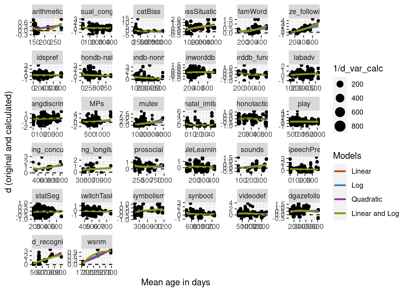
We ran mixed effects regressions where meta-analysis (data set) was included as a random intercept for our four models. We then ran Chi-squared tests to compare the different models to one another. Model comparison found the quadratic model to be a better fit than the linear model and the logarithmic model, but no difference between the linear and logarithmic model. The two predictor model (linear and log) also outperformed both the single predictor linear model and the single predictor logarithmic model.
lin_lmer <- lmer(d_calc ~ mean_age +
                (1 | dataset),
                weights = 1/d_var_calc,
                REML = F, data = metalab_data)

log_lmer <- lmer(d_calc ~ log(mean_age) +
                (1 | dataset),
                weights = 1/d_var_calc,
                REML = F, data = metalab_data)

quad_lmer <- lmer(d_calc ~ I(mean_age^2) +
                 (1 | dataset),
                 weights = 1/d_var_calc,
                 REML = F, data = metalab_data)

lin_log_lmer <- lmer(d_calc ~ mean_age + log(mean_age) +
                    (1| dataset),
                    weights = 1/d_var_calc,
                    REML = F, data = metalab_data)

kable(coef(summary(lin_lmer)))
| (Intercept) |
0.2657694 |
0.0460356 |
5.773127 |
| mean_age |
0.0000998 |
0.0000283 |
3.524569 |
kable(coef(summary(log_lmer)))
| (Intercept) |
0.3722238 |
0.0792106 |
4.6991675 |
| log(mean_age) |
-0.0100233 |
0.0111321 |
-0.9003996 |
kable(coef(summary(quad_lmer)))
| (Intercept) |
0.3115005 |
0.0461291 |
6.752799 |
| I(mean_age^2) |
0.0000000 |
0.0000000 |
1.167441 |
kable(coef(summary(lin_log_lmer)))
| (Intercept) |
0.4212793 |
0.0788645 |
5.341813 |
| mean_age |
0.0001291 |
0.0000308 |
4.186278 |
| log(mean_age) |
-0.0294871 |
0.0120632 |
-2.444380 |
kable(anova(lin_lmer, log_lmer))
| lin_lmer |
4 |
5068.739 |
5092.715 |
-2530.369 |
5060.739 |
NA |
NA |
NA |
| log_lmer |
4 |
5080.186 |
5104.162 |
-2536.093 |
5072.186 |
0 |
0 |
NA |
kable(anova(lin_lmer, quad_lmer))
| lin_lmer |
4 |
5068.739 |
5092.715 |
-2530.369 |
5060.739 |
NA |
NA |
NA |
| quad_lmer |
4 |
5079.621 |
5103.597 |
-2535.811 |
5071.621 |
0 |
0 |
NA |
kable(anova(log_lmer, quad_lmer))
| log_lmer |
4 |
5080.186 |
5104.162 |
-2536.093 |
5072.186 |
NA |
NA |
NA |
| quad_lmer |
4 |
5079.621 |
5103.597 |
-2535.811 |
5071.621 |
0.5645005 |
0 |
NA |
kable(anova(lin_lmer, lin_log_lmer))
| lin_lmer |
4 |
5068.739 |
5092.715 |
-2530.369 |
5060.739 |
NA |
NA |
NA |
| lin_log_lmer |
5 |
5064.807 |
5094.777 |
-2527.404 |
5054.807 |
5.931607 |
1 |
0.0148717 |
kable(anova(log_lmer, lin_log_lmer))
| log_lmer |
4 |
5080.186 |
5104.162 |
-2536.093 |
5072.186 |
NA |
NA |
NA |
| lin_log_lmer |
5 |
5064.807 |
5094.777 |
-2527.404 |
5054.807 |
17.37879 |
1 |
3.06e-05 |
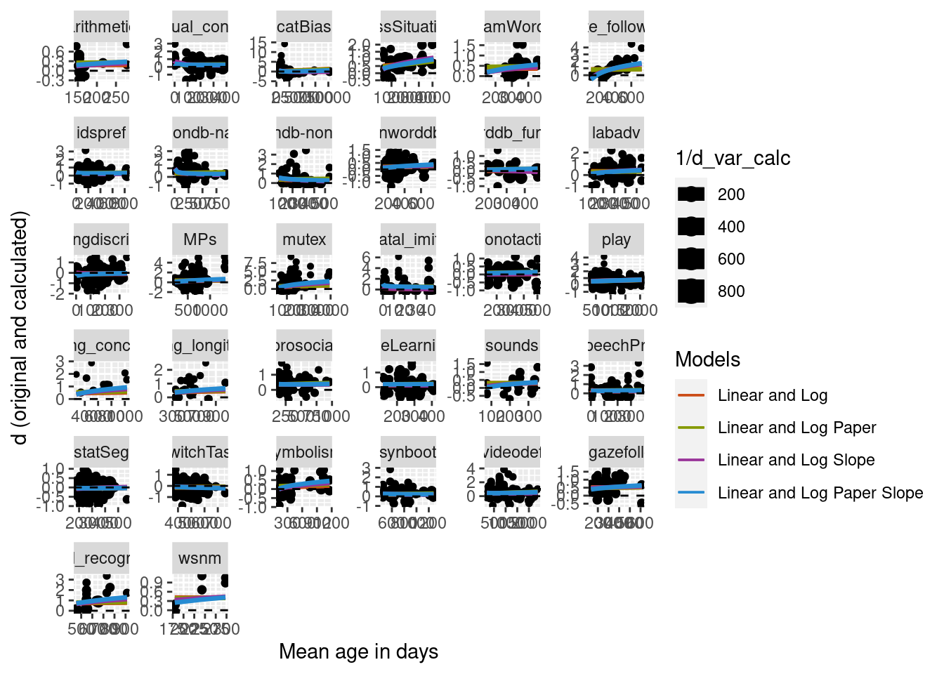
Focusing on the linear, log, and two predictor (linear and log) models, we built predictions for all complete meta-analyses. The plot separated by meta-analysis is presented below. The linear and two predictor models are pretty similar, mainly being different at very early ages.
metalab_data_preds <- metalab_data %>%
  select(dataset, short_name, d_calc, d_var_calc, mean_age, study_ID) %>%
  filter(complete.cases(.)) %>%
  mutate(lin_pred = predict(lin_lmer)) %>%
  mutate(log_pred = predict(log_lmer)) %>%
  mutate(lin_log_pred = predict(lin_log_lmer))
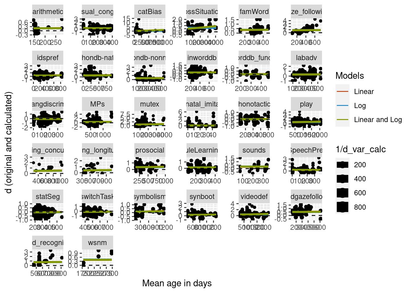
Overall this method looks pretty good. It seems like the linear predictor in the two predictor model is smoothing the logs at the edges, and the random effects are working to capture cross data set variability.
Complex random effects structure (nested paper effects)
We decided to expand our random effects structure to include paper (study_ID) nested in meta-analysis (data set) to capture the fact that a given meta-analysis has a specific set of papers, and may have multiple entries from the same paper. Here we focused on the two predictor model. The simpler random effects model from above is repeated here for easy comparison. A Chi-squared test finds a significant difference between the models, with the model with the more complex random effects structure having a lower AIC.
metalab_data <- metalab_data %>% select(d_calc, d_var_calc, mean_age, dataset, study_ID) %>% filter(complete.cases(.))

lin_log_paper_lmer <- lmer(d_calc ~ mean_age + log(mean_age) +
                          (1 | dataset / study_ID),
                          weights = 1/d_var_calc,
                          REML = F, data = metalab_data)

kable(coef(summary(lin_log_paper_lmer)))
| (Intercept) |
0.2779933 |
0.0959522 |
2.897206 |
| mean_age |
0.0001041 |
0.0000351 |
2.962590 |
| log(mean_age) |
0.0046257 |
0.0156777 |
0.295050 |
kable(coef(summary(lin_log_lmer)))
| (Intercept) |
0.4212793 |
0.0788645 |
5.341813 |
| mean_age |
0.0001291 |
0.0000308 |
4.186278 |
| log(mean_age) |
-0.0294871 |
0.0120632 |
-2.444380 |
kable(anova(lin_log_lmer, lin_log_paper_lmer))
| lin_log_lmer |
5 |
5064.807 |
5094.777 |
-2527.404 |
5054.807 |
NA |
NA |
NA |
| lin_log_paper_lmer |
6 |
4831.536 |
4867.500 |
-2409.768 |
4819.536 |
235.2713 |
1 |
0 |
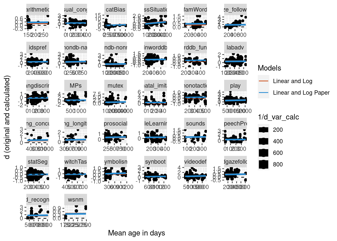
We then predicted from this new, more complex model and compare it to the model without the nested paper random effects structure. Initial testing found that including the nested random effect in the predict algorithm led to massive overfitting, so just the simple random effects structure was used to compute predictions. Below is the figure comparing the two curves. The curves are very similar, suggesting that while adding the nesting of paper does significantly improve the model, visually the difference is very small.
lin_log_paper_preds <- predict(lin_log_paper_lmer, re.form = ~ (1 | dataset))

metalab_data_preds <- metalab_data_preds %>%
  mutate(lin_log_paper_pred = lin_log_paper_preds)
Complex random effects structure (random slope)
Another way to make the random effects structure more complex is to add a random slope to the model. Two more models were built with a random slope by mean age log transformed, one without the nesting of paper, and one with the nesting of paper. Summaries of the new models with the random slope and the previous models without the random slope are below. Model comparison found that the model with nested structure and the slope was better than the simplest model (no nesting, no slope). The model with both the nested structure and the slope was also better than than the model with only the slope. Based on this it appears that the best model is one that includes both the nested random effects structure and a random slope of mean age log transformed.
lin_log_slope_lmer <- lmer(d_calc ~ mean_age + log(mean_age) +
                          (log(mean_age)| dataset),
                          weights = 1/d_var_calc,
                          REML = F, data = metalab_data)

lin_log_paper_slope_lmer <- lmer(d_calc ~ mean_age + log(mean_age) +
                          (log(mean_age)| dataset / study_ID),
                          weights = 1/d_var_calc,
                          REML = F, data = metalab_data)

kable(coef(summary(lin_log_slope_lmer)))
| (Intercept) |
-0.1692284 |
0.3833667 |
-0.4414271 |
| mean_age |
0.0000860 |
0.0000579 |
1.4857497 |
| log(mean_age) |
0.0718651 |
0.0678465 |
1.0592310 |
kable(coef(summary(lin_log_paper_slope_lmer)))
| (Intercept) |
-0.3787363 |
0.4301714 |
-0.8804311 |
| mean_age |
0.0001336 |
0.0000788 |
1.6953685 |
| log(mean_age) |
0.1099003 |
0.0772974 |
1.4217855 |
kable(coef(summary(lin_log_lmer)))
| (Intercept) |
0.4212793 |
0.0788645 |
5.341813 |
| mean_age |
0.0001291 |
0.0000308 |
4.186278 |
| log(mean_age) |
-0.0294871 |
0.0120632 |
-2.444380 |
kable(coef(summary(lin_log_paper_lmer)))
| (Intercept) |
0.2779933 |
0.0959522 |
2.897206 |
| mean_age |
0.0001041 |
0.0000351 |
2.962590 |
| log(mean_age) |
0.0046257 |
0.0156777 |
0.295050 |
kable(anova(lin_log_lmer, lin_log_slope_lmer))
| lin_log_lmer |
5 |
5064.807 |
5094.777 |
-2527.404 |
5054.807 |
NA |
NA |
NA |
| lin_log_slope_lmer |
7 |
4996.794 |
5038.752 |
-2491.397 |
4982.794 |
72.01276 |
2 |
0 |
kable(anova(lin_log_lmer, lin_log_paper_slope_lmer))
| lin_log_lmer |
5 |
5064.807 |
5094.777 |
-2527.404 |
5054.807 |
NA |
NA |
NA |
| lin_log_paper_slope_lmer |
10 |
4733.850 |
4793.789 |
-2356.925 |
4713.850 |
340.9573 |
5 |
0 |
kable(anova(lin_log_paper_lmer, lin_log_slope_lmer))
| lin_log_paper_lmer |
6 |
4831.536 |
4867.500 |
-2409.768 |
4819.536 |
NA |
NA |
NA |
| lin_log_slope_lmer |
7 |
4996.794 |
5038.752 |
-2491.397 |
4982.794 |
0 |
1 |
1 |
kable(anova(lin_log_paper_lmer, lin_log_paper_slope_lmer))
| lin_log_paper_lmer |
6 |
4831.536 |
4867.500 |
-2409.768 |
4819.536 |
NA |
NA |
NA |
| lin_log_paper_slope_lmer |
10 |
4733.850 |
4793.789 |
-2356.925 |
4713.850 |
105.6859 |
4 |
0 |
kable(anova(lin_log_slope_lmer, lin_log_paper_slope_lmer))
| lin_log_slope_lmer |
7 |
4996.794 |
5038.752 |
-2491.397 |
4982.794 |
NA |
NA |
NA |
| lin_log_paper_slope_lmer |
10 |
4733.850 |
4793.789 |
-2356.925 |
4713.850 |
268.9445 |
3 |
0 |
As before, predictions were built for the new models and plotted on the data. Overall the models do look pretty similar in terms of their predicted fit of the data.
lin_log_slope_preds <- predict(lin_log_slope_lmer, re.form = ~ (log(mean_age) | dataset))
lin_log_paper_slope_preds <- predict(lin_log_paper_slope_lmer, re.form = ~ (log(mean_age) | dataset))


metalab_data_preds <- metalab_data_preds %>%
  mutate(lin_log_slope_pred = lin_log_slope_preds) %>%
  mutate(lin_log_paper_slope_pred = lin_log_paper_slope_preds)
Subset to only those papers with multiple ages
One concern with using a random slope with meta-analysis nested by paper is that not all studies included more than one age group. To be sure that our random slope is really appropriate, here we look at only papers where more than one age group was tested.
Two age groups
To start we arbitrarily decided on two age groups, at least more than two months apart. Below we build a new model only looking at data where papers had at least two age groups. The structure of the model is the same as the model with papers nested in meta-analysis and a random slope of mean age log transformed.
multiage_data <- metalab_data_preds %>%
  group_by(dataset, study_ID) %>%
  mutate(count_ages = length(unique(floor(mean_age/2)))) %>%
  filter(count_ages > 1)

lin_log_paper_slope_multiage_lmer <- lmer(d_calc ~ mean_age + log(mean_age) +
                                     (log(mean_age) | dataset / study_ID),
                                     weights = 1/d_var_calc,
                                     REML = F, data = multiage_data)

kable(coef(summary(lin_log_paper_slope_multiage_lmer)))
| (Intercept) |
-0.4028799 |
0.4600573 |
-0.8757167 |
| mean_age |
0.0001897 |
0.0001020 |
1.8593404 |
| log(mean_age) |
0.1037670 |
0.0847375 |
1.2245709 |
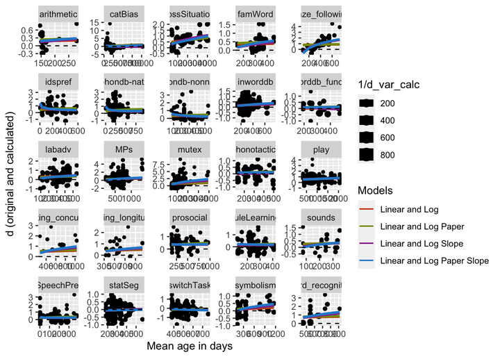
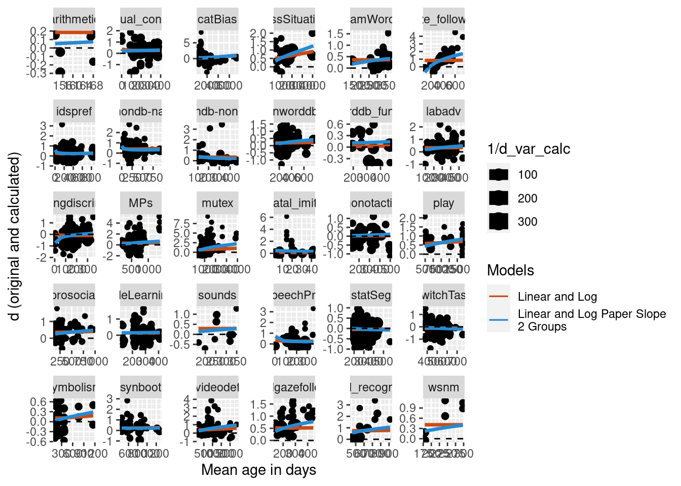
Predictions were calculated for the new model and visually compared to the simple model on the full data set with no nested random effects and no random slope. The plot below suggests that for this reduced data set, the addition of the nested random effects and random slope does differ greatly from the simpler model.
lin_log_paper_slope_multiage_preds <- predict(lin_log_paper_slope_multiage_lmer, re.form = ~ (log(mean_age)| dataset))

multiage_data <- multiage_data %>%
  ungroup %>%
  select(dataset, short_name, study_ID, d_calc, mean_age, d_var_calc, lin_log_pred) %>%
  mutate(lin_log_paper_slope_multiage_pred = lin_log_paper_slope_multiage_preds)
Three age groups
We also did the same analysis, but further reducing the data set to only papers that included at least three different age groups.
multiage_3_data <- metalab_data_preds %>%
  group_by(dataset, study_ID) %>%
  mutate(count_ages = length(unique(floor(mean_age/2)))) %>%
  filter(count_ages > 2)

lin_log_paper_slope_multiage_3_lmer <- lmer(d_calc ~ mean_age + log(mean_age) +
                                     (log(mean_age) | dataset / study_ID),
                                     weights = 1/d_var_calc,
                                     REML = F, data = multiage_3_data)

kable(coef(summary(lin_log_paper_slope_multiage_3_lmer)))
| (Intercept) |
-0.4158974 |
0.4996795 |
-0.8323283 |
| mean_age |
0.0002249 |
0.0001189 |
1.8910389 |
| log(mean_age) |
0.1015908 |
0.0916035 |
1.1090279 |
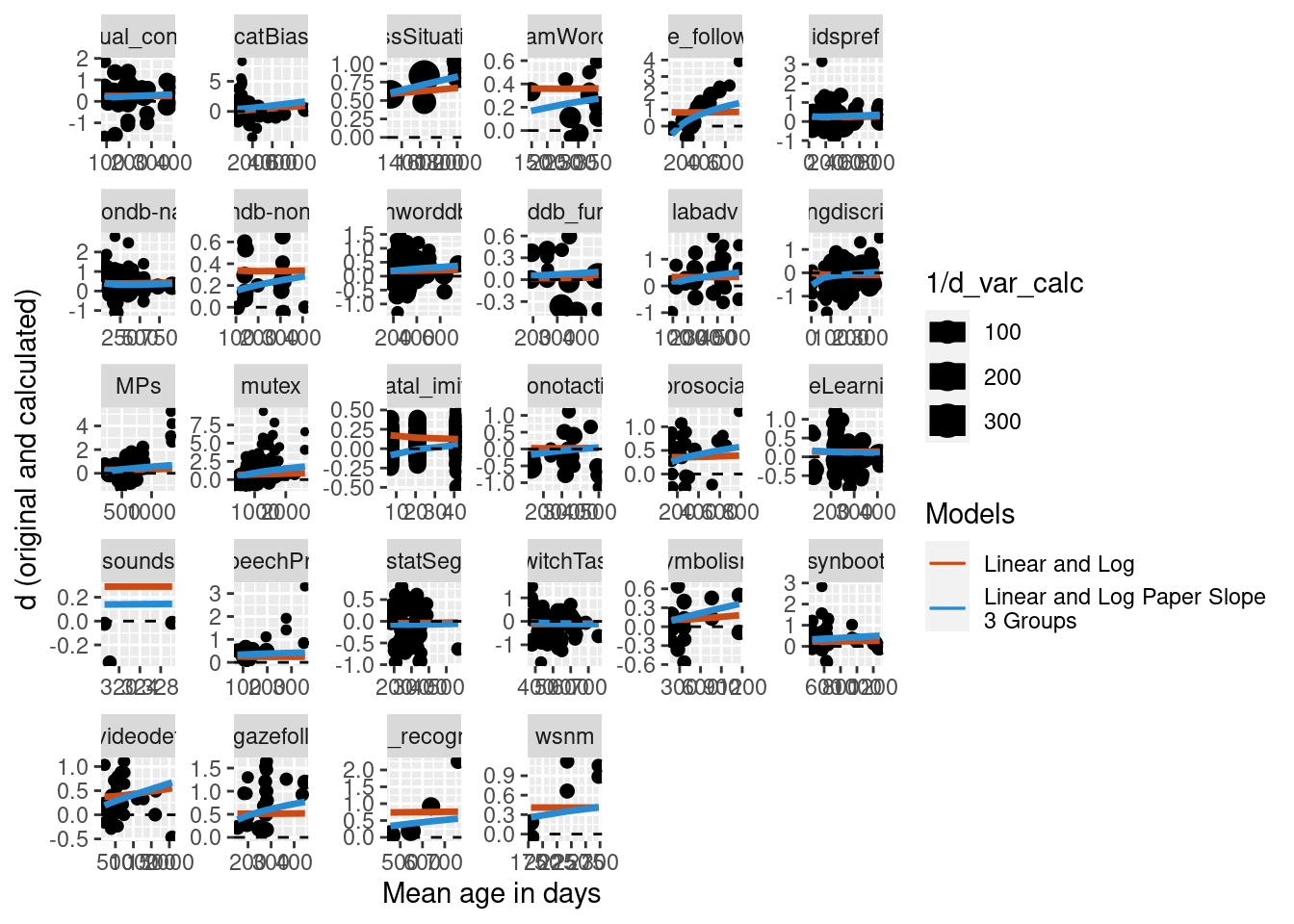
Predictions were calculated for the new model and visually compared to the simple model on the full data set with no nested random effects and no random slope. The plot below suggests that for this further reduced data set, the difference becomes the two models becomes even more apparent.
lin_log_paper_slope_multiage_3_preds <- predict(lin_log_paper_slope_multiage_3_lmer, re.form = ~ (log(mean_age)| dataset))

multiage_3_data <- multiage_3_data %>%
  ungroup %>%
  select(dataset, short_name, study_ID, d_calc, mean_age, d_var_calc, lin_log_pred) %>%
  mutate(lin_log_paper_slope_multiage_3_pred = lin_log_paper_slope_multiage_3_preds)
Conclusions
In this report we sought to find the best curve to describe developmental data. We found that, regarding predictors, the best fit of the data appears to be a model that includes both mean age and mean age log transformed as predictors. We further improved the curve by using complex random effects structures in our regressions. We found that a more complicated random effects structure was best by: 1) nesting paper in meta-analysis, and 2) including a random slope by mean age log transformed. This structure was most appropriate when we only looked at papers that had at least two or three age groups, to ensure the random slope applied to all data analyzed.